Data processing steps are explained by using the sample data sets stored in the SurfSeis "...\SampleData\" sub-folder. All acquisition parameters for the sample data sets are listed in Table 1.
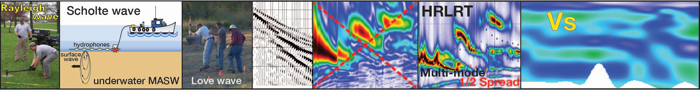
Figure 1a--Active MASW method. More information is available on "Active MASW."
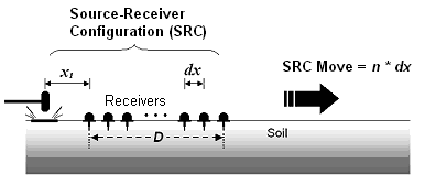
Figure 1b--Passive Remote MASW method. More information is available on "Passive Remote MASW."
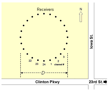
Figure 1c--Passive Roadside MASW method. More information is available on "Passive Roadside MASW."
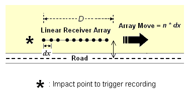
Table 1--Summary of sample data set parameters.
| Survey Type | Active MASW | Passive Remote MASW | Passive Remote MASW | Passive Roadside MASW |
|---|---|---|---|---|
| File Name(s) | "1011.dat"-"1022.dat" | "Passive-Cross.dat" | "Passive-Circular.dat" | "4000.dat"-"4009.dat" |
| Folder | "...\Active\" | "...\PassiveRemote\" | "...\PassiveRemote\" | "...\PassiveRoadside\" |
| Survey Purpose | 2-D Vs Profiling | 1-D Vs Profiling | 1-D Vs Profiling | 2-D Vs Profiling |
| Data Format | SEG-2 | KGS | KGS | SEG-2 |
| Acquisition | 24 channel | 48 channel | 24 channel | 48 channel |
| Source | 20-lb Hammer | Traffic | Traffic | 12-lb Hammer/Traffic |
| Receivers (Geophones) |
10-Hz (spike coupling) |
4.5-Hz (spike coupling) |
4.5-Hz (spike coupling) |
4.5-Hz (land streamer with 30 takeouts) |
| Receiver Array | Linear (roll along) | Cross (x-y) | Circular | Linear(roll along ) |
| Array Dimension (D) | 23 m | 115 m | 115 m | 35 m |
| Receiver Spacing (dx) | 1.22 m | 5 m | 15 m | 1.2 m |
| Source Offset (x1) | 1.22 m | N/A | N/A | 4.8 m |
| Receiver Array Move | 1 dx (1.22 m) | 0 | 0 | 4 dx (4.8 m) |
| Sampling Interval (dt) | 1 ms | 4 ms | 4 ms | 4 ms |
| Recording Time (T) | 2 sec | 20 sec | 120 sec | 120 sec |
| Record Numbers | 1011-1022 | 2000-2009 | 3000-3009 | 4000-4009 |
A summary of the entire procedure with a MASW method (active or passive) is displayed in the flowchart in Figure 2. Major changes and new features with this version are summarized as follows:
- Modules to process passive surface waves have been added in addition to the previously existing active module (Figure 1). Two different types of passive surveys are available: one, called the passive remote MASW method, uses a two-dimensional (2-D) receiver array and the other, called the passive roadside MASW method, uses the conventional 1-D linear array.
- The way dispersion analysis is executed has been changed so that the previous sequence of 'Preprocess-->Overtone-->Run-->Save' has been divided into two separate steps: (1) generation of dispersion image (called overtone, OT) data and (2) mouse-aided extraction of the dispersion curve from the image. The previous sequence, however, can still be accessed by right-clicking (instead of normal clicking) the 'Dispersion' button in the analysis menu when importing an input seismic file.
- A new mode of inversion has been added. This is a general Monte-Carlo method applied directly to the dispersion image (instead of the dispersion curve), seeking the best-matching solution through a random search. With this process, up to four modes of dispersion can be accounted for and all the parameters in a 5-layer earth model can be manually changed, if desired, to compare theoretical curve(s) with dispersion trend(s) in the background image.
Most (if not all) of the bugs existing in previous versions of SurfSeis have been fixed, thanks to the comments and reports from many practitioners who used SurfSeis to conduct the MASW method and who were very patient and always willing to help this quite new geophysical method still in its infancy evolve into a better form. We researchers at KGS sincerely appreciate your patience and assistance.
Figure 2--Flow chart of MASW processing steps.
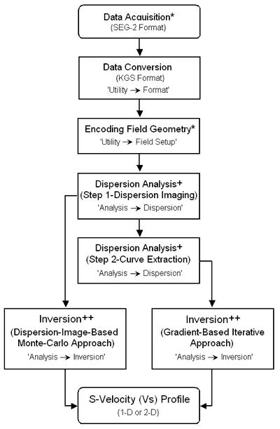
Data Processing
Step 1: Format (conversion from SEG-2 to KGS format)
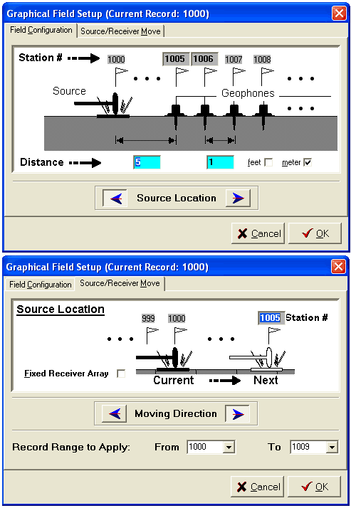
Step 2: Field Geometry Encoding
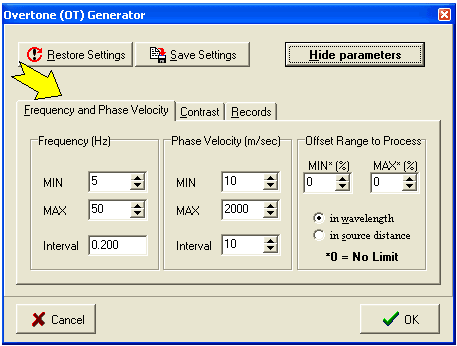
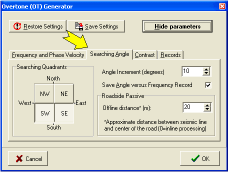
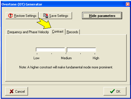
Step 3: Generation of Dispersion Image (called overtone) Data
Step 4: Extraction of Dispersion Curve(s)
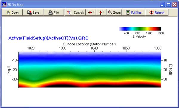
Step 5: Inversion of Curves for 2-D Vs Profile (Figure 5)
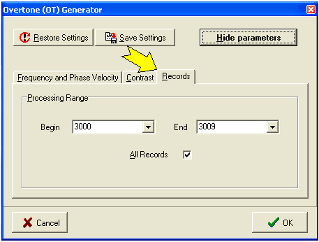
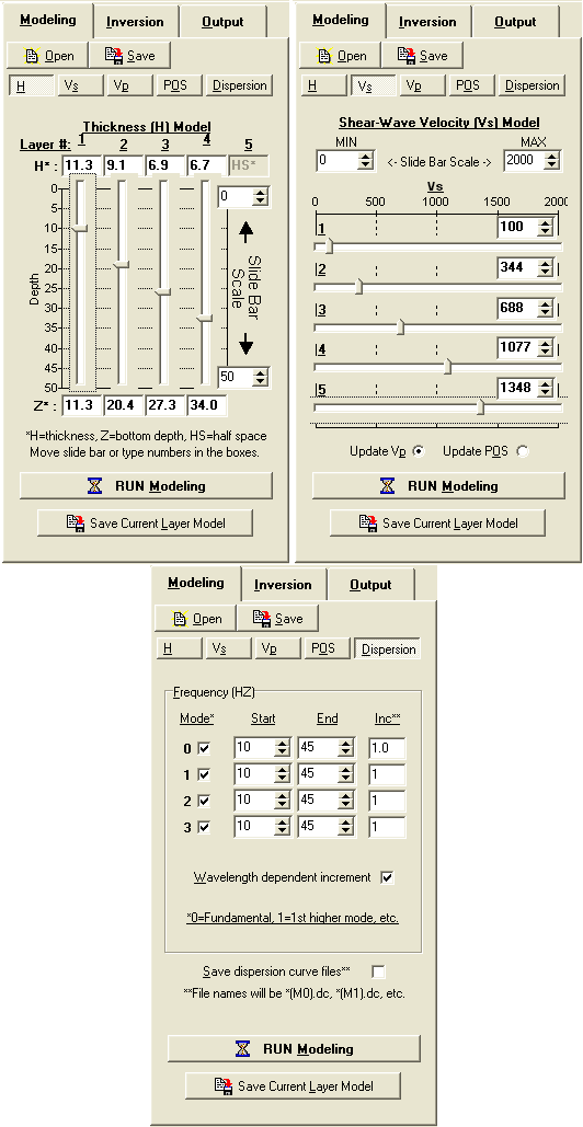
SurfSeis 2.0 Processing Steps
Field Setup (Active Survey)
Active Data Set Acquired in Roll-Along Mode
Encoding Field Geometry
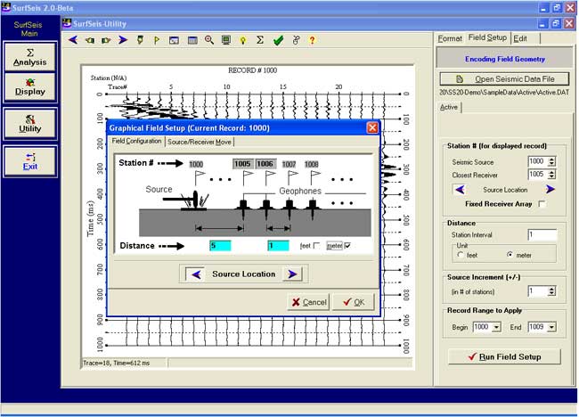
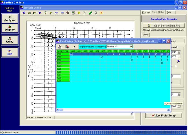
Source-receiver Station Table after Encoding
Field Setup (Passive Remote Survey)
X-Y Coordinate Setup for Each Receiver by Click and Drag
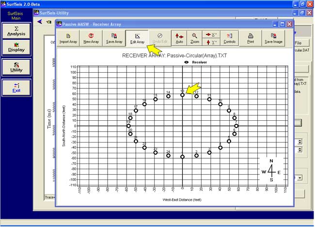
24-Channel Circular Array (After Completion of Setup)
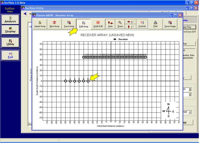
48-Channel Cross Array (Early Stage of Setup)
Field Setup (Passive Roadside Survey)
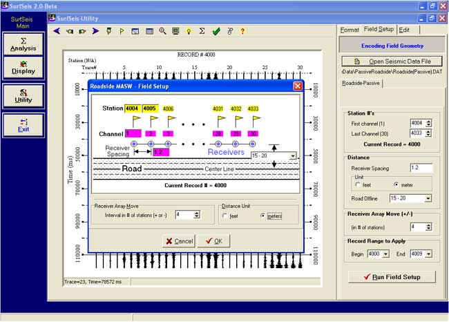
Passive Roadside Data Set Acquired in Roll-Along Mode
Encoding Field Geometry
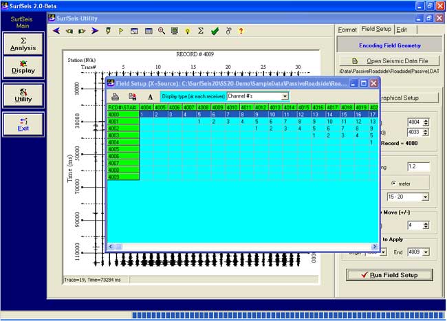
Source-receiver Station Table after Encoding
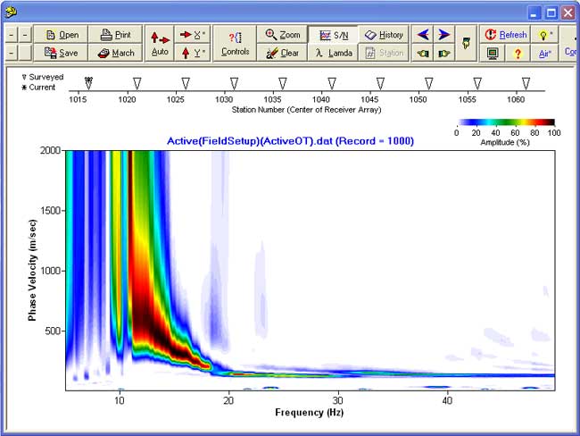
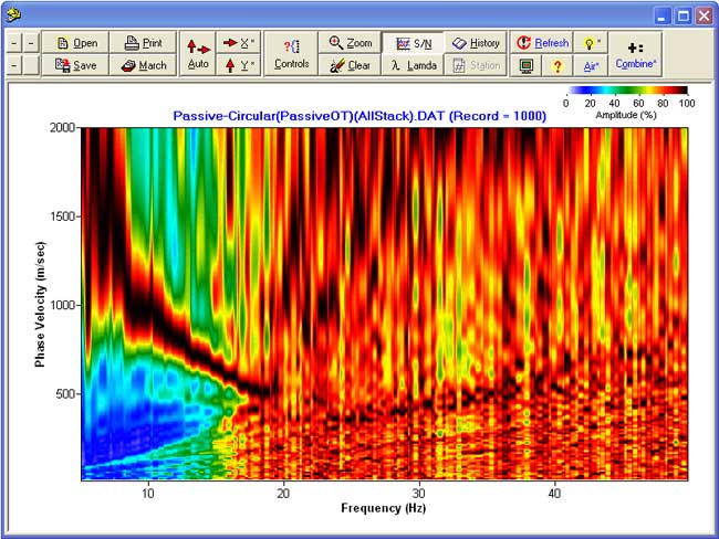
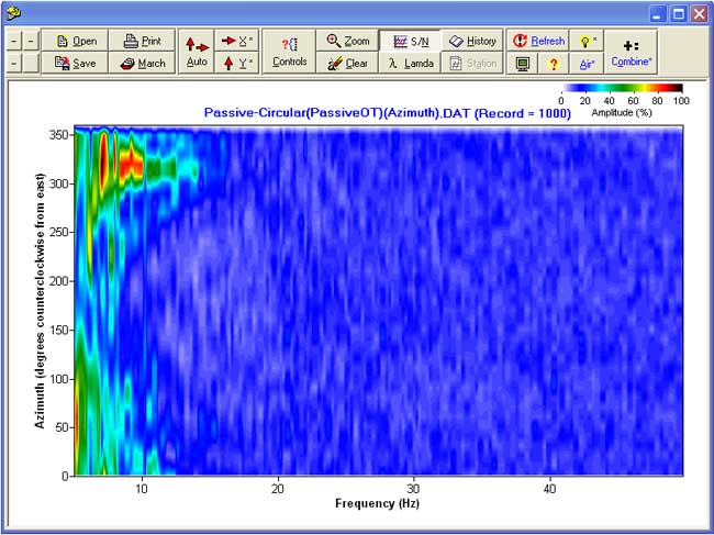
Dispersion Image Generation
Generation by 2-D Wavefield Transformation
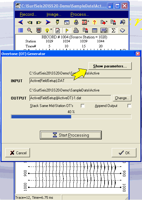
Controllable Processing Parameters
Active (A) and Passive (P)
Passive (P) Only
Active (A) and Passive (P)
Active (A) and Passive (P)
Dispersion Image
From Active Data
From Passive Remote Data
Azimuth Information of Passive Remote Data
Dispersion Curve Extraction
Setting Bounds by Mouse for Phase Velocity and Frequency Ranges
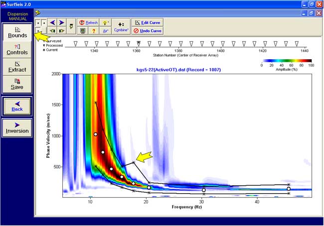
Extracting and Editing Dispersion Curve
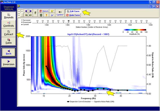
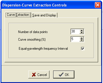
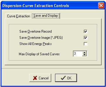
Controllable Parameters
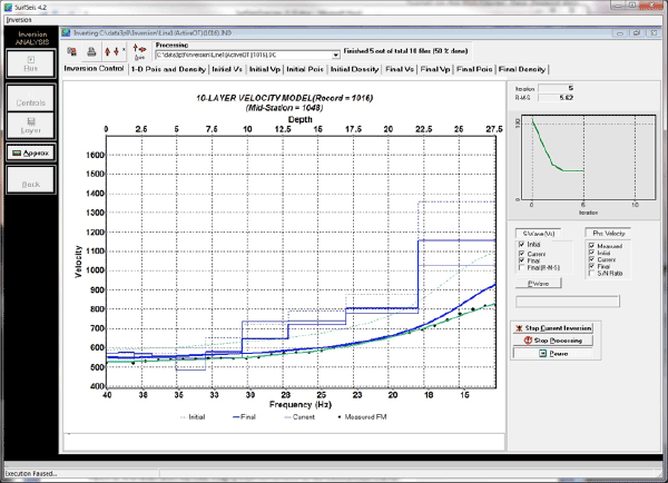
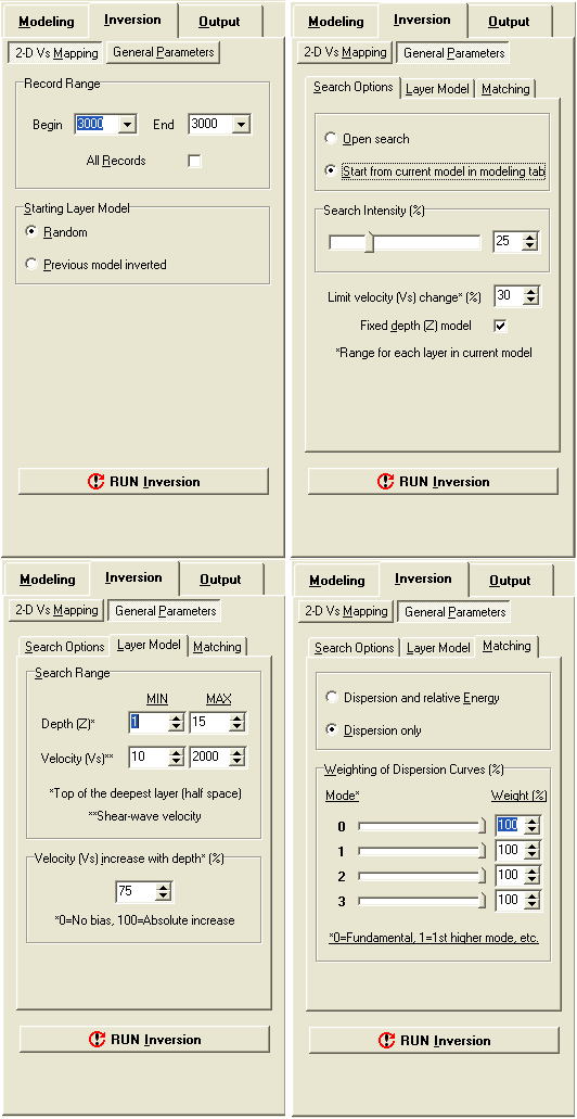
Inversion of Extracted Curves
Deterministic Inversion* of Dispersion Curves
*If all extracted dispersion-curves are of the fundamental mode of the Rayleigh wave only, this is the fastest, simplest, and most researched inversion approach to take. When using dispersion curves that have more than one modes (e.g., fundamental mode and one or more higher modes) possible inversion difficulties may arise (i.e., poor fit between observed and calculated curves, high RMS error) as a result of inaccurate mode interpretation. (Ivanov et al., 2010)
2-D Vs Profile from Inversion
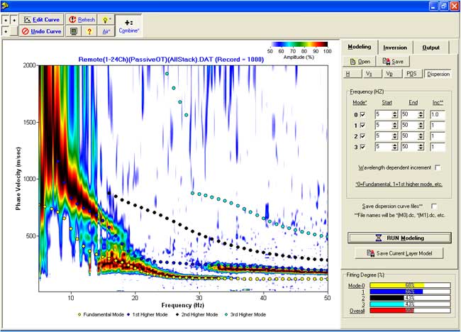
Modeling and Random Inversion on dispersion curve images
This tool allows the user to manually change model parameters, calculate up to 4 modes of the Rayleigh wave, and plot them on a dispersion-curve image for comparison.
Automatic Inversion by Monte-Carlo Approach for 2-D Vs Profile
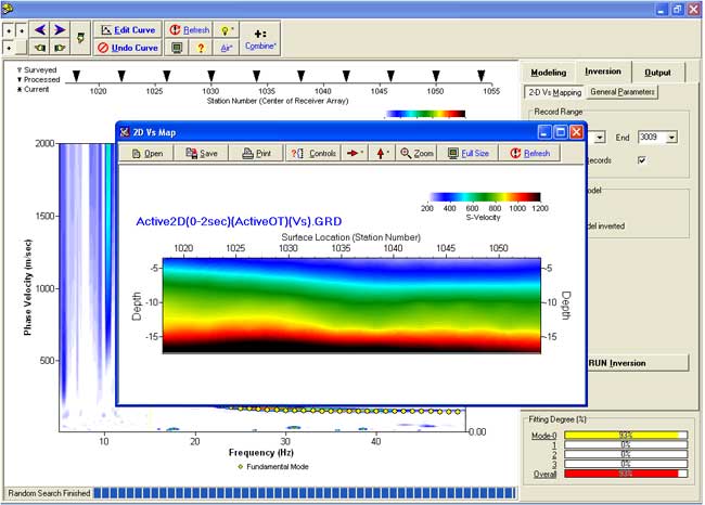
Random Inversion (Controls)
Monte-Carlo (a random) type of inversion can be applied by randomly changing the model parameters, calculating dispersion-curve points, and comparing them with the amplitudes on the dispersion-curve image. This approach can be very time consuming but it can be a useful research tool.
Note that different models can calculate sets of dispersion curve points from different modes that fit equally well the dispersion-curve image. Then mode interpretation can be of significance when choosing the solution.
As well, when performing modeling any type of inversion bear in mind that
- Dispersion-curve images can be different depending
- on the source offset and spread size,
- dispersion-curve-imaging algorithm and parameters.
- The use of HRLRT for dispersion curve imaging can be very useful for separating different modes, and understanding the possibilities for interpreting different trends on the dispersion- curve image (Ivanov et al., 2010).
Forward Modeling Portion
Inversion Portion
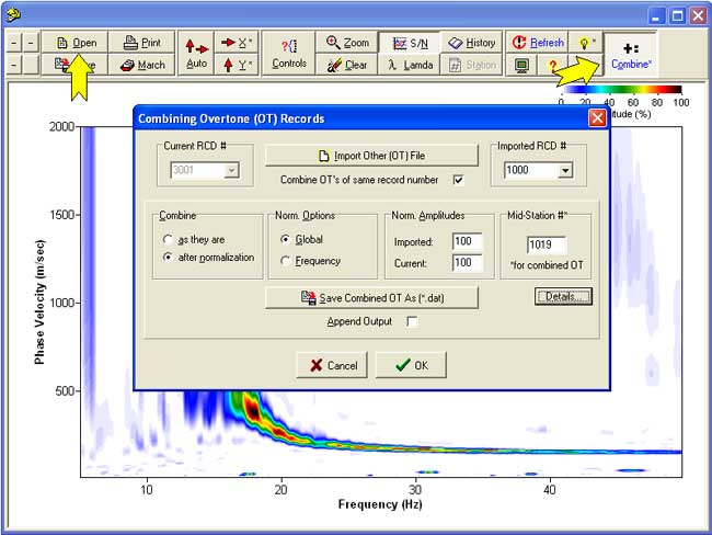
Combining Active and Passive Dispersion
To Increase Frequency (Depth) Range...
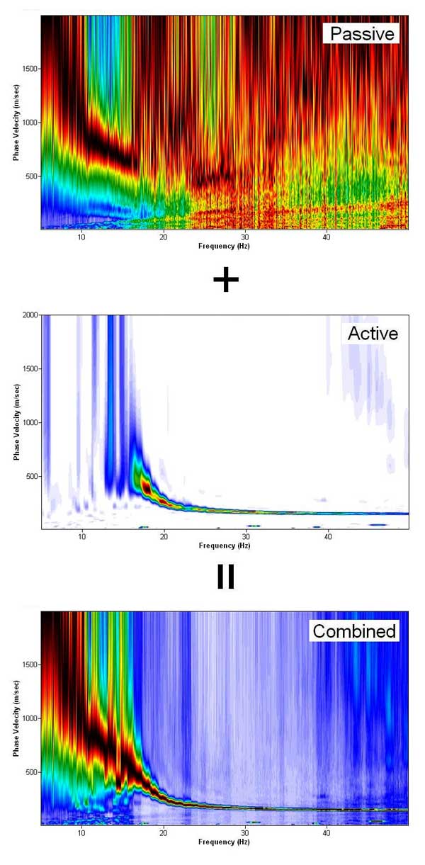
To Help Modal Identification...
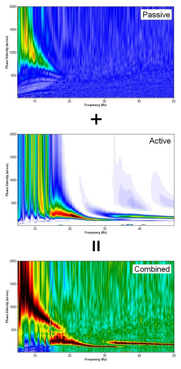
Opening an Active (or Passive) Image and then Passive (or Active) Image to Combine Together
References
Ivanov, J., R. D. Miller, and G. Tsoflias, 2008, Some Practical Aspects of MASW Analysis and Processing: Symposium on the Application of Geophysics to Engineering and Environmental Problems, 21, 1186-1198.
Ivanov, J., R. D. Miller, J. Xia, and S. Peterie, 2010, Multi-mode inversion of multi-channel analysis of surface waves (MASW) dispersion curves and high-resolution linear radon transform (HRLRT): 80th Annual International Meeting, SEG, Technical Program Expanded Abstracts, 29, 1902-1907.
Luo, Y. H., J. H. Xia, R. D. Miller, Y. X. Xu, J. P. Liu, and Q. S. Liu, 2009, Rayleigh-wave mode separation by high-resolution linear Radon transform: Geophysical Journal International, 179, 254-264.
Matheron, G., 1967, Kriging or Polynomial Interpolation Procedures--a Contribution to Polemics in Mathematical Geology: Canadian Mining and Metallurgical Bulletin, v. 60, no. 665, p. 33-58.
Miller, R. D., T. S. Anderson, J. Ivanov, J. C. Davis, R. Olea, C. Park, D. W. Steeples, M. L. Moran, and J. Xia, 2003, 3‐D characterization of seismic properties at the smart weapons test range, YPG: 73rd Annual International Meeting, SEG, Technical Program Expanded Abstracts, 22, 1195-1198.
Miller, R. D., J. Xia, C. B. Park, and J. M. Ivanov, 1999, Multichannel analysis of surface waves to map bedrock: The Leading Edge, 18, 1392–1396.
Olea, R. A., 1974, Optimal Contour Mapping Using Universal Kriging: Journal of Geophysical Research, 79, 695-702.
Park, C. B., and R. D. Miller, 2008, Roadside passive multichannel analysis of surface waves (MASW): Journal of Environmental and Engineering Geophysics, 13, 1-11.
Park, C. B., R. D. Miller, D. Laflen, C. Neb, J. Ivanov, B. Bennett, and R. Huggins, 2004, Imaging dispersion curves of passive surface waves: 74th Annual International Meeting, SEG, Expanded Abstracts, 23, 1357-1360.
Park, C. B., R. D. Miller, N. Ryden, J. Xia, and J. Ivanov, 2005, Combined use of active and passive surface waves: Journal of Environmental and Engineering Geophysics, 10, 323-334.
Park, C. B., R. D. Miller, and J. Xia, 1998, Imaging dispersion curves of surface waves on multi-channel record 68th Annual International Meeting, SEG, Expanded Abstracts, 1377-1380.
Park, C. B., R. D. Miller, and J. H. Xia, 1999, Multichannel analysis of surface waves: Geophysics, 64, 800-808.
Song, Y. Y., J. P. Castagna, R. A. Black, and R. W. Knapp, 1989, Sensitivity of near‐surface shear‐wave velocity determination from rayleigh and love waves: 59th Annual International Meeting, SEG, Expanded Abstracts, 8, 509-512.
Xia, J. H., R. D. Miller, and C. B. Park, 1999, Estimation of near-surface shear-wave velocity by inversion of Rayleigh waves: Geophysics, 64, 691-700.
Xia, J. H., Y. X. Xu, and R. D. Miller, 2007, Generating an image of dispersive energy by frequency decomposition and slant stacking: Pure and Applied Geophysics, 164, 941-956.