Introduction to MASW
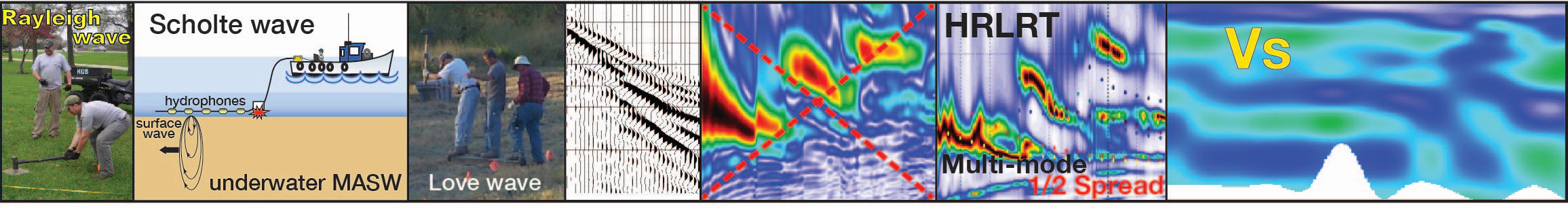
Rayleigh-, Scholte-, and Love- waves
Kansas Geological Survey is the birth place of the multichannel analysis of surface waves (MASW) method research efforts originated at the Kansas in the late 80s. It originally focused on analyzing Rayleigh surface waves, which are typically acquired using vertical sources and receivers. Later Scholte waves (aka underwater MASW) and Love-waves were naturally included with appropriate adjustments in the acquisition and analysis.
Four Steps of MASW Process
The entire MASW procedure usually consists of four steps (Miller et al., 1999):
- Acquiring multichannel records (or shot gathers),
- Dispersion-curve imaging and curves estimations (from each record)
- Inversion of dispersion curves to obtain 1D (depth) Vs profiles for each record
- Assembling multiple 1D results into 2D or 3D images.
1. Acquiring multichannel records (or shot gathers)
Depending on the nature of the seismic source the MASW method can be categorized as Active or Passive.
1.1 The Active MASW (Figure 1), which was introduced in The Leading Edge by Miller et al. (1999), uses user-controlled seismic sources (e.g., a sledge hammers, weight drop, charges, etc.) and typically a linear receiver array (aka seismic spread) collecting data in a roll-along mode (i.e., moving the whole acquisition system with a regular step). The Active MASW often is the preferred approach because of the ability to control the source distance to the seismic spread. The latter can affect the ability to observe low or high frequencies of the fundamental mode of the surface wave (and thus "see" deeper or shallower) depending on the source being relatively far or near, accordingly (Ivanov et al., 2008).
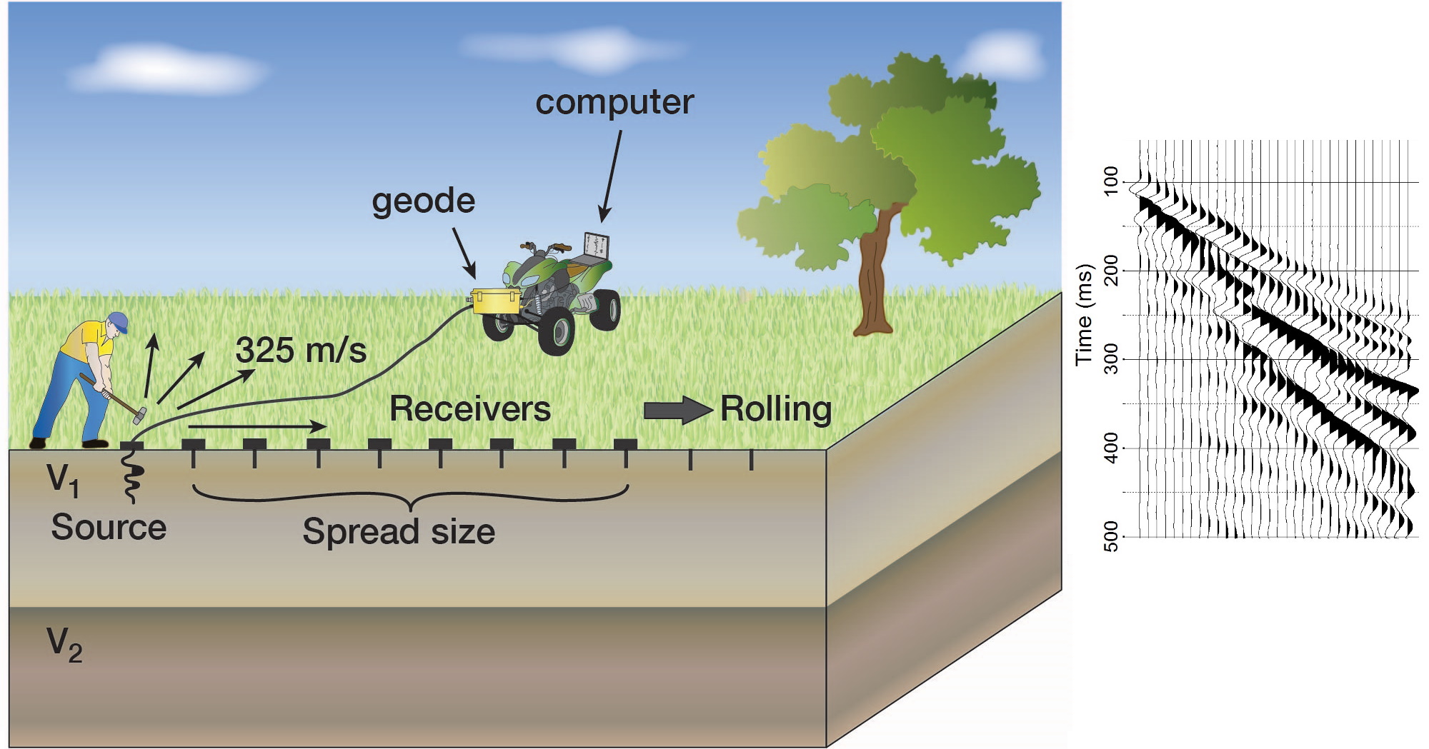
Figure 1. Active MASW a) a data acquisition diagram showing a source, receivers, and rolling (moving them all) direction and b) the signal from all receivers making a seismic shot record.
1.2 The Passive MASW method utilizes surface waves generated by uncontrolled and possibly unknown sources of seismic energy. One of the main benefits of using passive sources is the likelihood of observing lower frequencies (than the "Active" can provide) and thus extend the depth of investigation (e.g., for Vs30)
1.2.1 A linear (i.e., horizontal 1D) receiver array
1.2.1.1 pointing into the direction of a known source location (Figure 2) in the absence of other, oblique-angle sources is considered to be the optimal case (Ivanov et al., 2013; Morton et al., 2018).
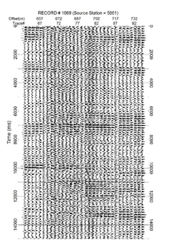
Figure 2. Passive data from a linear array.
1.2.1.2 Another 1D receiver array possibility it to place it next, parallel to a road the Passive Roadside MASW (Park and Miller, 2008).
1.2.2 Using a two-dimensional (2D) receiver array (Figure 3), aka The Passive Remote MASW (Park et al., 2004; Park et al., 2005) assumes far sources and does not require knowledge about their location. This results in the most accurate evaluation of shear-wave velocity (Vs) when the source direction is unknown but is at the expense of more intensive field operation and the need for securing the space for the receiver array.

Figure 3. Circular and rectangular receiver arrays with a smaller nested into a larger array targeting relatively shorter and longer surface-wave wavelengths.
2. Dispersion-curve imaging and estimations
Dispersion properties of all types of waves (both body and surface waves) are imaged through a 2D wavefield-transformation method (Song et al., 1989; Park et al., 1998; Luo et al., 2008), which can be viewed as a remapped versions of an FK transform (Ivanov et al., 2015). Each multichannel record is converted into a dispersion-curve image (a.k.a. Overtone), on which different dispersion patterns can be identified or interpreted (Figure 3). Then, the necessary dispersion features (e.g., the fundamental mode of the Rayleigh wave, the first higher mode, etc.) can be interpreted and estimated following a specific energy trend. Selected points (Figure 4) can be saved as a dispersion-curve file, which can be then inverted for a 1D Vs profile.
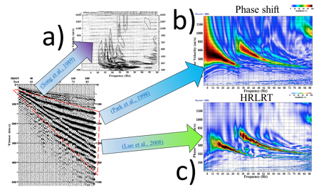
Figure 4. Three dispersion-curve images from a seismic record using a) conventional FK transform remapping, b) the phase-shift method, and c) the HRLRT transform.
3. Inversion of dispersion curves to obtain 1D (depth) Vs profiles for each record
The goal of the surface-wave inversion is to find a Vs layer model whose calculated dispersion curve would reasonably match well the observed dispersion-curve points (Figure 5).
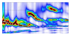
Figure 5. Dispersion-curve points picked on a HRLRT image from an "extra-short" spread record.
The inversion starts with an initial Vs model from which a dispersion curve is calculated and compared to the picked dispersion-curve points. Based on their difference the inversion algorithm estimates Vs model modification to obtain another Vs model. This new model is used to calculate another dispersion curve, which is compared to the picked dispersion-curve points, etc. This iterative process continues until the calculated curve matches reasonably well with the picked dispersion-curve points (Figure 6).
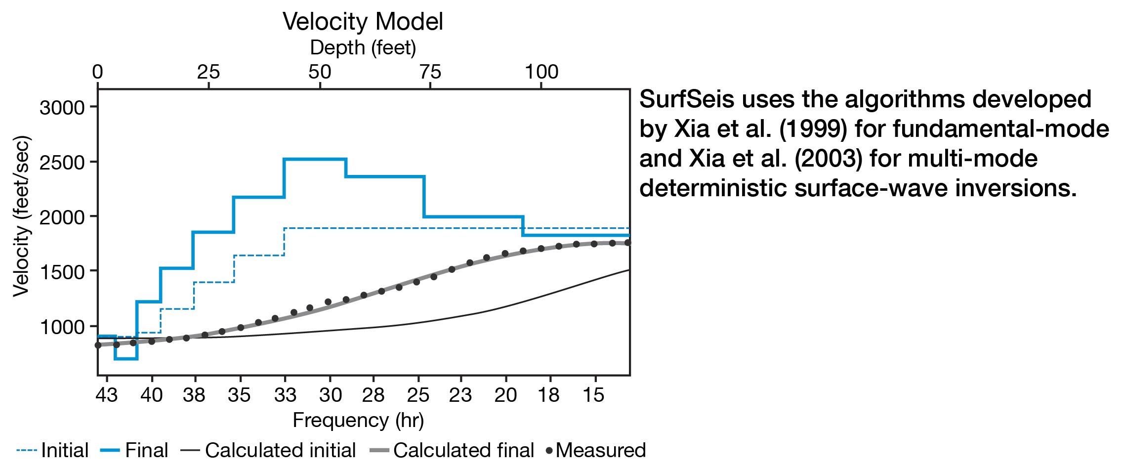
Figure 6. Dispersion-curve inversion. Black dots indicate the measured dispersion curve, the thin blue dashed step line shows the initial layer model, the thin black line shows the calculated dispersion curve from the initial model, the thick blue line shows the final layer model, and the thick black line the shows the calculated dispersion curve from the final model.
4. Assembling multiple 1D results into 2D or 3D images.
The final step is assembling the multiple 1D Vs final results into a 2D image, cross-sections (Miller et al., 1999), 3D volumes (Miller et al., 2003), etc. The surface location of each 1D Vs profile is obtained from the middle of the receiver spread (Figure 7).
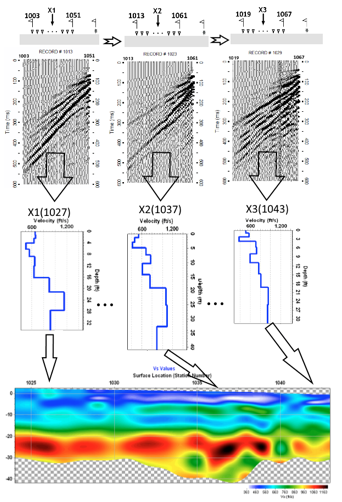
Figure 7. Assembling 1D Vs results from records with different locations.
References
Ivanov, J., R. D. Miller, and G. Tsoflias, 2008, Some Practical Aspects of MASW Analysis and Processing: Symposium on the Application of Geophysics to Engineering and Environmental Problems, 21, 1186-1198.
Ivanov, J., J. T. Schwenk, S. L. Peterie, and J. Xia 2013, The joint analysis of refractions with surface waves (JARS) method for finding solutions to the inverse refraction problem: The Leading Edge, 32, 692-697.
Ivanov, J., R. D. Miller, S. Morton, and S. Peterie, 2015, Dispersion-curve imaging considerations when using multichannel analysis of surface wavee (MASW) method, Symposium on the Application of Geophysics to Engineering and Environmental Problems 2015, 556-566.
Luo, Y. H., J. H. Xia, R. D. Miller, Y. X. Xu, J. P. Liu, and Q. S. Liu, 2008, Rayleigh-wave dispersive energy imaging using a high-resolution linear Radon transform: Pure and Applied Geophysics, 165, 903-922.
Miller, R. D., J. Xia, C. B. Park, and J. M. Ivanov, 1999, Multichannel analysis of surface waves to map bedrock: The Leading Edge, 18, 1392-1396.
Miller, R. D., T. S. Anderson, J. Ivanov, J. C. Davis, R. Olea, C. Park, D. W. Steeples, M. L. Moran, and J. Xia, 2003, 3-D characterization of seismic properties at the smart weapons test range, YPG: 73rd Annual International Meeting, SEG, Technical Program Expanded Abstracts, 22, 1195-1198.
Morton, S. L., J. Ivanov, S. L. Peterie, R. D. Miller, R. L. Parsons, and A. J. Livers-Douglas, 2018, Time-lapse monitoring of subsidence features within the Hutchinson Salt in Kansas, SEG Technical Program Expanded Abstracts 2018, 2642-2646.
Park, C. B., R. D. Miller, and J. Xia, 1998, Imaging dispersion curves of surface waves on multi-channel record 68th Annual International Meeting, SEG, Expanded Abstracts, 1377-1380.
Park, C. B., R. D. Miller, D. Laflen, C. Neb, J. Ivanov, B. Bennett, and R. Huggins, 2004, Imaging dispersion curves of passive surface waves: 74th Annual International Meeting, SEG, Expanded Abstracts, 23, 1357-1360.
Park, C. B., R. D. Miller, N. Ryden, J. Xia, and J. Ivanov, 2005, Combined use of active and passive surface waves: Journal of Environmental and Engineering Geophysics, 10, 323-334.
Park, C. B., and R. D. Miller, 2008, Roadside passive multichannel analysis of surface waves (MASW): Journal of Environmental and Engineering Geophysics, 13, 1-11.
Song, Y. Y., J. P. Castagna, R. A. Black, and R. W. Knapp, 1989, Sensitivity of near‐surface shear‐wave velocity determination from rayleigh and love waves: 59th Annual International Meeting, SEG, Expanded Abstracts, 8, 509-512.
Xia, J. H., R. D. Miller, and C. B. Park, 1999, Estimation of near-surface shear-wave velocity by inversion of Rayleigh waves: Geophysics, 64, 691-700.
Xia, J. H., R. D. Miller, C. B. Park, and G. Tian, 2003, Inversion of high frequency surface waves with fundamental and higher modes: Journal of Applied Geophysics, 52, 45-57.