Passive Remote MASW
A passive surface wave survey with a 2-D receiver array (Figure 1) will give the most accurate evaluation of dispersion trend (Park and Miller, 2006). This mode of survey, however, requires a wide area for the 2-D array, which must be deployed some distance away (remote) from points of surface wave generation to meet the plane-wave-propagation assumption. In the case of roadside survey, this distance can be a fraction (e.g., 20%) of the dimension (D) of the receiver array. Procedures in data acquisition and processing are explained.
Figure 1--Passive Remote MASW method.
Receiver Array
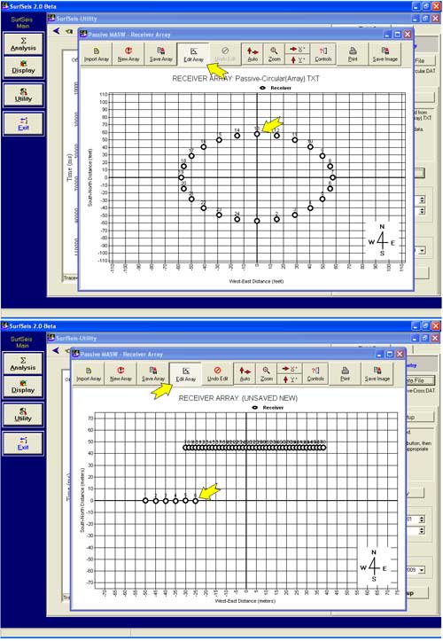
Any type of 2-D array of fairly symmetric shape can be used (Figure 2). An array of significant asymmetric shape, for example an elliptical or elongated rectangular shape, is not recommended due to bias toward a specific direction of incoming surface waves that do not necessarily coincide with the actual direction of major surface wave energy. Common array types may include the circle, cross, square, triangular, random, etc.
Figure 2--Possible types of receiver arrays for passive remote MASW survey.
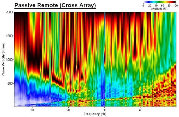
A detailed study comparing each different type of array and its effect on dispersion analysis has not been reported yet, as far as systematic and scientific perspectives are concerned. Intensive modeling tests performed at Kansas Geological Survey, however, indicated an insignificant difference between different types insofar as the symmetry of the array is maintained. It is, therefore, the convenience of field operation that determines the specific type to be used. Field experiments with circular and cross arrays indicated the circle may result in dispersion images with a slightly higher resolution and better definition (Figure 3).
Figure 3a--Circular array and associated phase-frequency plot.
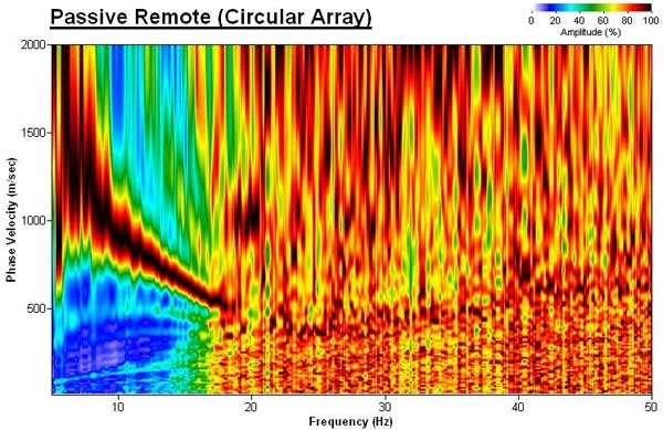
Figure 3b--Cross array and associated phase-frequency plot.
Array Dimension (D) and Receiver Spacing (dx)
Array dimension (D) is directly related to the longest wavelength (![]() ) that can be analyzed, which in turn determines the maximum depth of investigation (zmax):
) that can be analyzed, which in turn determines the maximum depth of investigation (zmax):
![]()
On the other hand, (minimum if uneven) receiver spacing (dx) is related to the shortest wavelength (![]() ) and therefore the shallowest resolvable depth of investigation (zmin).
) and therefore the shallowest resolvable depth of investigation (zmin).
![]()
Data Acquisition
Parameters described here are those most commonly used at KGS, and by no means represent a required set of values. A slight variation in any parameter can always be expected.
Recording Parameters
Sampling interval of 4 ms (dt = 4 ms) and total recording time of 30 sec (T = 30 sec) are most commonly used at KGS when surveys are performed inside the city of Lawrence. Total recording time (T) is determined in such a way that there is at least one occurrence of passive surface wave generation during recording. Therefore, it can be reduced or increased depending on local situations related to the surface wave generation. In case of surveys near roads, for example, there should be a vehicle passing near the survey area at least once during recording.
The longer T is not always better. This is because the chance of recording surface waves generated at different locations (azimuths) on the road increases as well and it will in general degrade the data processing resolution unless those locations are well apart in azimuth (for example, 90° or more). If the main source point is fixed in location, however, the longer T will be the better. A fixed source point of major surface waves is observed when you hear a loud jolting sound coming from nearly the same spot (azimuth) on the road as vehicles pass over.
Vertical stacking during recording is strongly discouraged (unless T is significantly limited) because it will increase the change of recording multi-azimuth surface waves previously explained. Instead, we recommend saving individual records separately. Then, the dispersion imaging process can be applied to individual records and then these image records can be vertically stacked together to enhance the definition of the image. However, if T is limited to a shorter time (e.g., < 30 sec) by the recording device, then a few times of vertical stacking (e.g., stacking 10-sec recording three times) may be necessary either during recording or post-acquisition stage.
D and dx will approximately determine the minimum number of channels needed. In any case, however, more channels will be an advantage that can increase the resolution of dispersion processing to a certain degree. 48 channels are most desirable for a survey aiming at zmax ≈ 100 m. When fewer than 48 channels are available (e.g., 24), data acquisition can proceed with an array of smaller dimension (e.g., D = 25 m) and then with progressively larger dimensions (e.g., D = 50 m, 75 m, 100 m, etc.) to cover a broader range of wavelengths (![]() ). In this case, dispersion image data sets processed separately can be combined together to construct a broader-band dispersion image.
). In this case, dispersion image data sets processed separately can be combined together to construct a broader-band dispersion image.
If dynamic range is a controllable option with a recording device, choosing the highest value, along with the highest gain if available also, will always be a benefit.
Necessity of Separate Active Survey
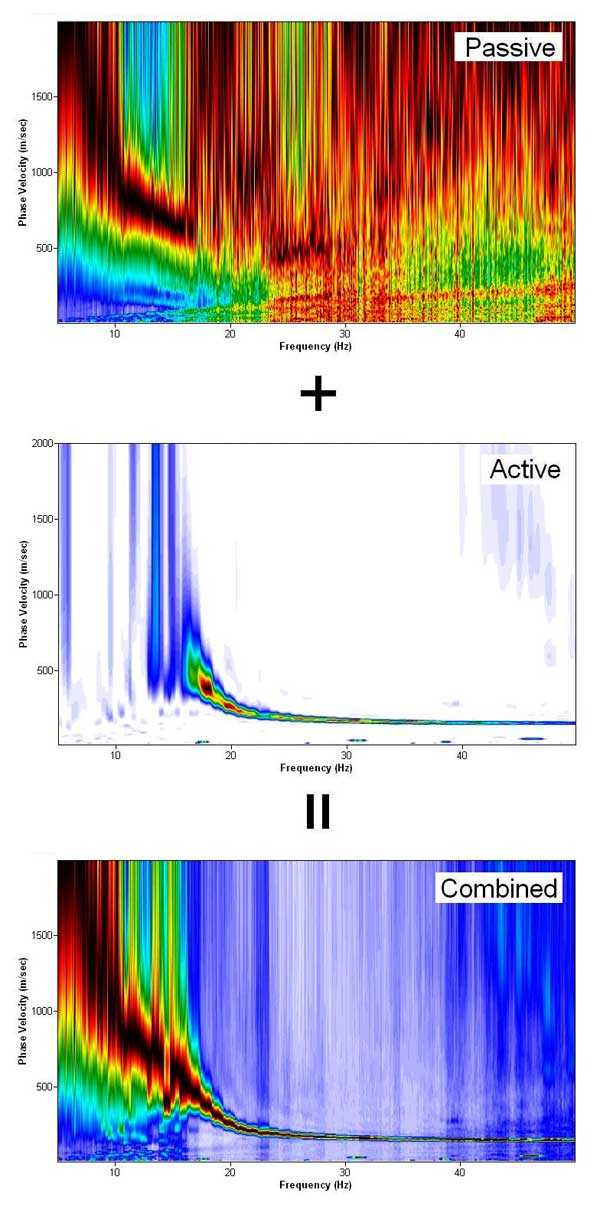
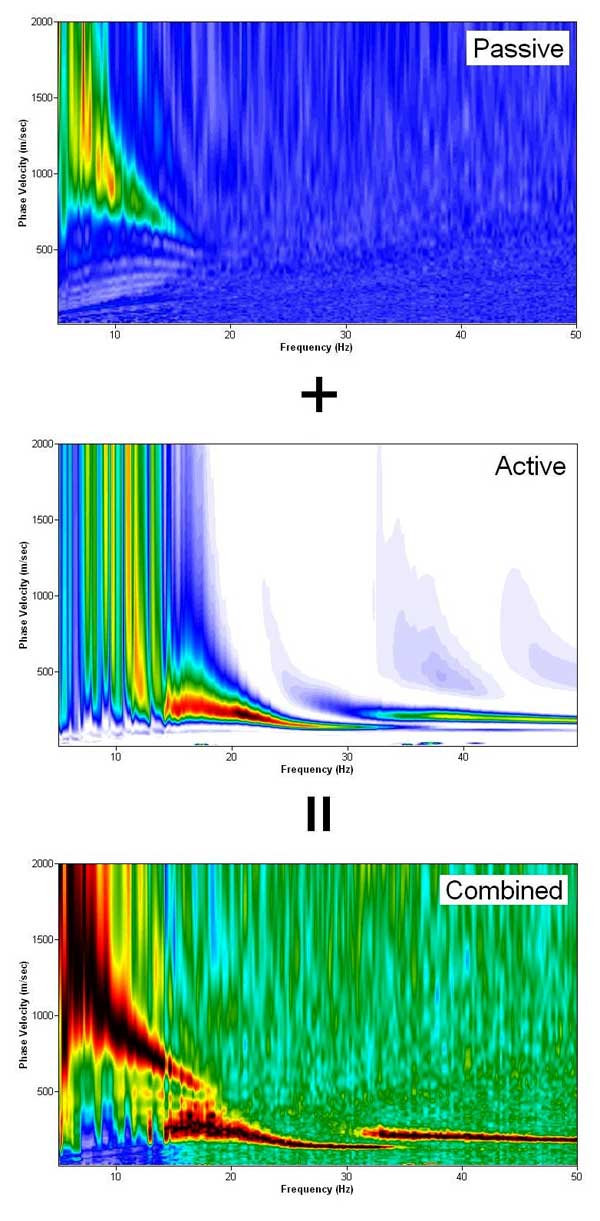
Because a passive survey usually operates with much a larger receiver spacing than normally used in an active survey, a processed dispersion image usually lacks information at shallower (higher) depths (frequencies). Although in theory this missing information can be filled by multiple surveys of progressively smaller dimensions (D's), higher frequency components of passive surface waves may not be recorded effectively because of their relatively rapid attenuation properties. The best way would be to perform a separate active survey, preferably at the array center, using a sledge hammer. Then, two separate dispersion image data sets can be combined together to form a broader-band image (Figure 4). Combining active and passive dispersion images can also help modal identification.
Figure 4--Combination of Active and Passive datasets.
An alternative approach instead of a separate active survey would be to apply active impact(s) at a place close to (but outside) the receiver array during the recording of a passive record. If this is the case, however, please note that
- Analyzed shear-velocity (Vs) information at shallow depths can only be associated with those near-surface materials near the impact point.
- Analyzed dispersion trend for those high frequencies generated by the active source can be slightly distorted (at most 10%) because of a violation of the plane-wave assumption.
- Dispersion image for those low-frequency passive waves can be adversely influenced and result in a degraded definition or slightly distorted trend or both.
A more detailed study on this issue has been planned at KGS and will be reported soon. Reports of experimental results from practitioners are always welcome.
Data Processing
Step 1: Format (conversion from SEG-2 to KGS format)
Step 2: Field Geometry Encoding
Step 3: Generation of Dispersion Image (called overtone) Data
Step 4: Extraction of Dispersion Curve(s)
Step 5: Inversion of Curves for 2-D Vs Profile
References
Park, C.B., and Miller, R.D., 2006, Roadside passive MASW: Proceedings of SAGEEP, April 2-6, 2006, Seattle, Washington. [PDF available online, 1.3 MB]