Active MASW

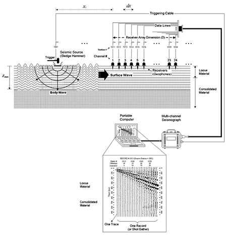
This is the most common type of MASW survey that can produce a 2-D Vs profile (Park et al., 1999). The overall setup is illustrated in Figure 1. The maximum depth of investigation (z_max) that can be achieved is usually in 10-30 m range, but this can vary with sites and types of active sources used. Field procedures and data processing steps are briefly explained below. Some of the field parameters, for example, source offset (x₁) and receiver spacing (dx), are described based on the most recent research results and therefore may be different from those previously reported.

Figure 1--Active MASW method.

Surface waves are best generated over a 'flat' ground at least within one receiver-spread length (D) (Figure 2). Then, overall topographic variation within an entire survey line should not matter. However, any surface relief whose dimension is greater than, say, 10% of D will cause a significant hindrance to surface wave generation.

Figure 2--Flat or gentle slopes will be suitable for Active MASW. However, topography can interfere with surface-wave propagation.

Data Acquisition

The following describes most of parameters related to data acquisition. These are the parameters most commonly used at KGS and by no means represent a required set of values. A slight variation in any parameter can always be expected.

Source

A fairly heavy sledge hammer (e.g., 10 lb) will be a good choice, although any other type (e.g., a weight drop) that can deliver more impact power into ground can be an advantage over a sledge hammer because of its potential to generate lower (longer) frequencies (wavelengths) of surface waves. The gain from using these other sources is often not enough to warrant the cost of equipment and inconvenience in field operation. Using an impact plate (also called base plate) will help the source impact point become less intrusive into soil. Detailed study on the role of the base plate in surface wave generation has not yet been reported and needs to be undertaken in the near future. Recently, it has been reported that a non-metallic plate (e.g., a firm rubber plate) can generate noticeably stronger energy at the lower frequency (e.g., < 10 Hz) part of surface waves than the conventional metallic plate.

Vertical stacking with multiple impacts can suppress ambient noise significantly and is therefore always recommended, especially if the survey takes place in an urban area. The optimum number of stacking impacts can be determined when there is little change in signal-to-noise ratio (S/N) in the displayed seismic record during the stacking. We often use 3-5 vertical stacks at Kansas Geological Survey. This number, however, should increase as the ambient noise level increases and/or total receiver array length (D) increases.

Receivers

Low-frequency (e.g., 4.5 Hz) geophones are always recommended. Effectiveness of somewhat higher-frequency (e.g., 10-20 Hz) phones, however, is often comparable to that of much lower-frequency ones. Vertical (instead of horizontal) phones must be used. Although spike-coupled geophones always give the highest sensitivity, the coupling provided by a land streamer can be equally well suited with a significant convenience in field operation.

Field Geometry

Length of the receiver spread (D) (Figure 1) is directly related to the longest wavelength () that can be analyzed, which in turn determines the maximum depth of investigation (z_max):

On the other hand, (minimum if uneven) receiver spacing (dx) is related to the shortest wavelength () and therefore the shallowest resolvable depth of investigation (z_min).

In practice, however, (therefore D) in an active survey is usually limited by the seismic source as it is the most governing factor. It is usually in a few tens of meters (e.g., < 30 m) in most cases.

The source offset (x1) controls the degree of contamination by the near-field effects. Its optimum value has been a debatable subject. We, however, suggest a value of about 20% of D (e.g., x₁=5 m when D=25 m). A large value of x₁ (e.g., > 10 m) and a large D (e.g., > 100 m) will increase the risk of higher-mode domination and reduce S/N for the fundamental mode. The following is most recommended:

Interval (dSRC) of Source-Receivers Configuration (SRC) Move

An interval between 1dx-12dx is recommended. 4dx is most commonly used in the case of 24-channel acquisition.

Recording Parameters

A one millisecond (dt = 1 ms) of sampling interval is most common with a 2-sec total recording time (T = 2 sec). Use a smaller dt (e.g., 0.5 ms) if any body-wave processing (e.g., refraction and reflection) is planned as by-product(s). In the case of extremely low velocities (e.g., Vs < 100 m/sec), a longer T (e.g., 4 sec) will be a better choice. In any case, an excessively long T (e.g., T ≥ 5 sec) is discouraged as it can increase the chance of recording ambient noise (e.g., traffic). Usually, 24-channel acquisition will be optimal. If 48-channel acquisition is available, it is recommended to shorten dx rather than to increase D.

Data Processing

Step 1: Format (conversion from SEG-2 to KGS format)

Step 2: Field Geometry Encoding

Step 3: Generation of Dispersion Image (called overtone) Data

Step 4: Extraction of Dispersion Curve(s)

Step 5: Inversion of Curves for 2-D Vs Profile (Figure 5)

References

Park, C.B., Miller, R.D., and Xia, J., 1999, Multichannel analysis of surface waves (MASW); Geophysics, 64, 800-808. [PDF available online, 1.3 MB]

References

Heisey, J. S., K. H. Stokoe, W. R. Hudson, and A.H. Meyer, 1982, Determinatin of in situ shear-wave velocity from spectral anaylysis of surface waves: Center for Transportation Research, The University of Texas at Austin, 256-2.
Ivanov, J., R. D. Miller, and G. Tsoflias, 2008, Some Practical Aspects of MASW Analysis and Processing: Symposium on the Application of Geophysics to Engineering and Environmental Problems, 21, 1186-1198.
Miller, R. D., T. S. Anderson, J. Ivanov, J. C. Davis, R. Olea, C. Park, D. W. Steeples, M. L. Moran, and J. Xia, 2003a, 3-D characterization of seismic properties at the smart weapons test range, YPG: 73rd Annual International Meeting, SEG, Technical Program Expanded Abstracts, 22, 1195-1198.
Miller, R. D., K. G. Park, J. Ivanov, C. B. Park, D. Laflen, and R. F. Ballard, 2003b, A 2-C Towed Geophone Spread for Variable Surface Conditions: Symposium on the Application of Geophysics to Engineering and Environmental Problems, 16, 1276-1284.
Miller, R. D., J. Xia, C. B. Park, and J. M. Ivanov, 1999, Multichannel analysis of surface waves to map bedrock: The Leading Edge, 18, 1392-1396.
Park, C. B., R. D. Miller, and J. Xia, 2001, Offset and Resolution of Dispersion Curve in Multichannel Analysis of Surface Waves (MASW): Symposium on the Application of Geophysics to Engineering and Environmental Problems, 14, SSM4.
Park, C. B., R. D. Miller, and J. H. Xia, 1999, Multichannel analysis of surface waves: Geophysics, 64, 800-808.
Rix, G. J., and A. E. Leipski, 1991, Accuracy Accuracy and resolution of surface wave inversion; in, B. S. K. a. B. G.W., ed., Proceedings of Sessions Sponsored by the Geotechnical Engineering (Geotechnical special publication) American Society of Civil Engineers, 17-23.
Roesset, J. M., D. W. Chang, K. H. Stokoe II, and M. Aouad, 1989, Modulus and thickness of the pavement surface layer from SASW tests: Transportation Research Record, 1260, 53-63.
Stokoe, K. H., II , G. W. Wright, J. A. Bay, and M. R. Roesset, 1994, Characterization of geotechnical sites by SASW method; in, R. D. Woods, ed., Geophysical characterization of sites: A. A. Balkema, 15-25.
Xia, J., R. D. Miller, C. B. Park, J. A. Hunter, and J. B. Harris, 2000, Comparing shear-wave velocity profiles from MASW with borehole measurements in unconsolidated sediments, Fraser River Delta, B.C., Canada: Journal of Environmental and Engineering Geophysics, 1, 1-13.
Xu, Y. X., J. H. Xia, and R. D. Miller, 2006, Quantitative estimation of minimum offset for multichannel surface-wave survey with actively exciting source: Journal of Applied Geophysics, 59, 117-125.
Zhang, S. X., L. S. Chan, and J. H. Xia, 2004, The selection of field acquisition parameters for dispersion images from multichannel surface wave data: Pure and Applied Geophysics, 161, 185-201.