The first version of the SurfSeis software (v. 1.0) was released in 2000 for the application of the multichannel analysis of surface waves (MASW) method on seismic data. Developed at the Kansas Geological Survey (KGS), the MASW method consists of four main components (Miller et al., 1999): roll-along data acquisition, dispersion-curve imaging (Song et al., 1989; Park et al., 1998; Xia et al., 2007; Luo et al., 2009), dispersion-curve inversion to obtain a 1-D shear-wave velocity (Vs) profile (Xia et al., 1999), and assembling multiple 1-D results into 2-D or 3-D images (Miller et al., 1999; Miller et al., 2003) using interpolation algorithms (Matheron, 1967; Olea, 1974).
Initially the MASW method was developed for data acquired using active seismic sources, a.k.a. "Active MASW" (Miller et al., 1999; Park et al., 1999). The same technique was later extended to the application on seismic data from passive sources, a.k.a. "Passive MASW" (Park et al., 2004; Park et al., 2005a; Park and Miller, 2008; Ivanov et al., 2013; Ivanov et al., 2017a). The next versions of the software - SurfSeis 2, 3, 4, 5, and 6 - have included new features that take into account new research and methodological developments (http://www.kgs.ku.edu/software/surfseis/pubs_year.html), as well as users' demands for more options and improved user interface.
The main set of manuals distributed with the software was developed for SurfSeis version 1.5. The manuals for the following versions focus only on the new developments.
SurfSeis 2 manual (Manual2.05.pdf) has been prepared mainly to explain the possibilities of using the passive MASW approach, forward dispersion-curve modeling (dispersion-curve values estimations using a 1-D velocity model) and display on dispersion-curve images (a.k.a., Overtone images), and random Monte Carlo inversion on dispersion-curve images. The SurfSeis 2 manual can serve as a stand-alone manual for both active and passive MASW methods for those who have previous experience in seismic data acquisition and data processing in either body- or surface-wave methods.
SurfSeis 3 manual (Manual3.05.pdf) provides information on how to pick and invert higher modes of the Rayleigh surface wave (in addition to the conventional fundamental-mode use), discusses the new menu system developed to provide an alternate friendly access to SurfSeis' processes (in addition to the previously existing button-driven interface), and informs about the new software licensing/protection method using a USB key (a.k.a., hardware key, dongle, etc.).
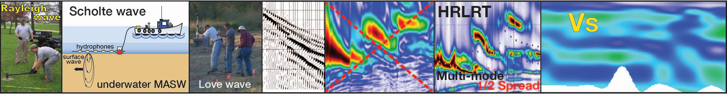
SurfSeis 4 manual (SurfSeis4UserManual.pdf) talks about the next set of newly developed features designed to provide more tools that can contribute to a higher quality of surface-wave analysis, such as sliding-window passive-data dispersion-curve imaging, flexible 2D a-priori initial-model parameters input (i.e., compressional velocity (Vp), Poisson's ratio, and density), ongoing-inversion 2D monitoring, etc. As well, the v4 manual demonstrates the sharper dispersion-curve imaging abilities when using the high-resolution linear radon transform (Luo et al., 2009), which is optionally available in SurfSeis 4.2.
SurfSeis 5 manual (SurfSeis5UserManual.pdf) discusses how to observe variable elevations and maximum-depth with 2-D imaging. We find the latter especially helpful for interpretation purposes and avoiding hard-to-notice extrapolation areas. HRLRT is now available for passive-data dispersion-curve imaging, which we often find significantly superior over other imaging methods. HRLRT was also made available for single-record processing (typically useful for initial data testing and evaluations). Modeling and Random Inversion on dispersion curve images (a.k.a. frequency - velocity spectrum and "effective mode") was expanded to use up to 20 layers and input from .lst results. Applicable for Rayleigh and optional for Love waves. Scholte-wave [a.k.a., underwater (Kaufmann et al., 2005; Park et al., 2005b) MASW] modeling and inversion, random (on dispersion curve images) and deterministic (i.e., regular). Love-wave (Xia et al., 2012b; Ivanov et al., 2017b) modeling and inversion, random (on dispersion curve images) and deterministic (i.e., regular), which is optionally available in SurfSeis 5.1 and SurfSeis 5.3.
SurfSeis 6 manual (SurfSeis6UserManual.pdf) indicates how to apply constrained inversion (e.g., with data measurements from wells), stitch dispersion-curve images for improving low and high frequencies and horizontal resolution of the final Vs estimates Advanced Kriging capabilities provide optimized statistical models to choose from for interpolation. Qs (and conditionally Qp) estimations (Xia et al., 2012a; Ivanov et al., 2014; Feigenbaum et al., 2016) from Rayleigh-wave attenuation measurements with estimating attenuation curves conventionally and/or after special focusing filtered that are used for inverting for Qs (Qp), which is optionally available in SurfSeis 6 versions 6.4 through 6.7.
References
Feigenbaum, D., J. Ivanov, R. Miller, S. Peterie, and S. Morton, 2016, Near-surface Qs estimations using multichannel analysis of surface waves (MASW) and the effect of nonfundamental mode energy on Q estimation: An example from Yuma proving ground, Arizona, SEG Technical Program Expanded Abstracts 2016, 4971-4976.
Ivanov, J., B. Leitner, W. T. Shefchik, T. J. Schwenk, and S. L. Peterie, 2013, Evaluating hazards at salt cavern sites using multichannel analysis of surface waves: The Leading Edge, 32, 289-305.
Ivanov, J., R. D. Miller, S. L. Peterie, and G. Tsoflias, 2014, Near-surface Qs and Qp estimations from Rayleigh waves using multi-channel analysis of surface waves (MASW) at an Arctic ice-sheet site, SEG Technical Program Expanded Abstracts 2014, 2006-2012.
Ivanov, J., R. Miller, D. Feigenbaum, and J. Schwenk, 2017a, Benefits of using the high-resolution linear Radon transform with the multichannel analysis of surface waves method, SEG Technical Program Expanded Abstracts 2017, 2647-2653.
Ivanov, J., R. D. Miller, D. Feigenbaum, S. L. C. Morton, S. L. Peterie, and J. B. Dunba, 2017b, Revisiting levees in southern Texas using Love-wave multichannel analysis of surface waves with the high-resolution linear Radon transform: Interpretation, 5, T287-T298.
Kaufmann, R. D., J. H. Xia, R. C. Benson, L. B. Yuhr, D. W. Casto, and C. B. Park, 2005, Evaluation of MASW data acquired with a hydrophone streamer in a shallow marine environment: Journal of Environmental and Engineering Geophysics, 10, 87-98.
Luo, Y. H., J. H. Xia, R. D. Miller, Y. X. Xu, J. P. Liu, and Q. S. Liu, 2009, Rayleigh-wave mode separation by high-resolution linear Radon transform: Geophysical Journal International, 179, 254-264.
Matheron, G., 1967, Kriging or Polynomial Interpolation Procedures - a Contribution to Polemics in Mathematical Geology: Canadian Mining and Metallurgical Bulletin, 60, 1041-&.
Miller, R. D., J. Xia, C. B. Park, and J. M. Ivanov, 1999, Multichannel analysis of surface waves to map bedrock: The Leading Edge, 18, 1392-1396.
Miller, R. D., T. S. Anderson, J. Ivanov, J. C. Davis, R. Olea, C. Park, D. W. Steeples, M. L. Moran, and J. Xia, 2003, 3-D characterization of seismic properties at the smart weapons test range, YPG: 73rd Annual International Meeting, SEG, Technical Program Expanded Abstracts, 22, 1195-1198.
Olea, R. A., 1974, Optimal Contour Mapping Using Universal Kriging: Journal of Geophysical Research, 79, 695-702.
Park, C. B., R. D. Miller, and J. Xia, 1998, Imaging dispersion curves of surface waves on multi-channel record 68th Annual International Meeting, SEG, Expanded Abstracts, 1377-1380.
Park, C. B., R. D. Miller, and J. H. Xia, 1999, Multichannel analysis of surface waves: Geophysics, 64, 800-808.
Park, C. B., R. D. Miller, D. Laflen, C. Neb, J. Ivanov, B. Bennett, and R. Huggins, 2004, Imaging dispersion curves of passive surface waves: 74th Annual International Meeting, SEG, Expanded Abstracts, 23, 1357-1360.
Park, C. B., R. D. Miller, N. Ryden, J. Xia, and J. Ivanov, 2005a, Combined use of active and passive surface waves: Journal of Environmental and Engineering Geophysics, 10, 323-334.
Park, C. B., R. D. Miller, J. Xia, J. Ivanov, G. V. Sonnichsen, J. A. Hunter, R. L. Good, R. A. Burns, and H. Christian, 2005b, Underwater MASW to evaluate stiffness of water-bottom sediments: The Leading Edge, 24, 724-728.
Park, C. B., and R. D. Miller, 2008, Roadside passive multichannel analysis of surface waves (MASW): Journal of Environmental and Engineering Geophysics, 13, 1-11.
Song, Y. Y., J. P. Castagna, R. A. Black, and R. W. Knapp, 1989, Sensitivity of near-surface shear-wave velocity determination from rayleigh and love waves: 59th Annual International Meeting, SEG, Expanded Abstracts, 8, 509-512.
Xia, J. G., Y. X. Xu, R. D. Miller, and J. Ivanov, 2012a, Estimation of near-surface quality factors by constrained inversion of Rayleigh-wave attenuation coefficients: Journal of Applied Geophysics, 82, 137-144.
Xia, J. H., R. D. Miller, and C. B. Park, 1999, Estimation of near-surface shear-wave velocity by inversion of Rayleigh waves: Geophysics, 64, 691-700.
Xia, J. H., Y. X. Xu, and R. D. Miller, 2007, Generating an image of dispersive energy by frequency decomposition and slant stacking: Pure and Applied Geophysics, 164, 941-956.
Xia, J. H., Y. X. Xu, Y. H. Luo, R. D. Miller, R. Cakir, and C. Zeng, 2012b, Advantages of Using Multichannel Analysis of Love Waves (MALW) to Estimate Near-Surface Shear-Wave Velocity: Surveys in Geophysics, 33, 841-860.