
![]()
Prev Page--Hydrogeology, Hydrogeochemistry || Next Page--Calibration
Part B
Digital Simulation of the Pawnee Valley Alluvial Aquifer
Introduction
The rate of water-level decline is the most important piece of information needed by the groundwater management districts in the study area. In particular, it is of paramount importance to know how rapidly the resource is being depleted, where and when water-level declines will seriously affect existing investments, and what impacts alternative developments or management practices will have on the system. Digital simulation offers a reliable means for evaluating the effects of various development alternatives on an aquifer system such as the Pawnee valley alluvial aquifer.
A simulation model is a simplification or abstraction of a complex physical reality and its processes. There is no need to elaborate on the fact that most real systems, and certainly the aquifer system, are indeed complicated beyond our capability to describe them and to treat them exactly as they are. Simplifications are necessary. They take the form of a set of assumptions that should be kept in mind whenever the model is being employed in the course of investigations. On the basis of these simplifying assumptions, a model of an investigated groundwater system is constructed. Because groundwater flow obeys a well-defined set of physical laws which can be expressed mathematically, it is possible to replace actual problems in groundwater flow by analogous mathematical problems {models). This is the reason why models are always presented in the form of a set of mathematical equations, the solution of which yields the behavior of the considered system. In almost all cases, the equations are balance equations based on the principle of conservation of mass and on Darcy's law.
Obviously, it is impossible either to carry out experiments and tests in the aquifer itself to determine its response to various management alternatives or to make comparisons among responses to different possible alternatives to determine the most desirable one. Whenever the treatment of real systems or phenomena is impossible or the cost of such treatment is prohibitive, models of the considered system or phenomena are introduced. Instead of treating the real system, we manipulate its model and use the results of these manipulations in order to make decisions regarding the operation of the real system.
Groundwater Simulation Model
The mathematical equation describing the two-dimensional ground- water flow through an areally extensive aquifer is given by the following partial differential equation (Bittinger and others, 1967)
![]()
where, K = hydraulic conductivity [L/T]
b = saturated thickness [L]
H = hydraulic head [L]
S = storativity or specific yield (dimensionless)
Q = net withdrawal flow [L3 / T)
Δx, Δy = incremental distances
x,y = space dimensions
t = time
[L] denotes units of length, [T] units of time
This equation is based on the continuity equation and Darcy's law and is consistent with the Dupuit assumptions. The Dupuit assumptions are (l) the velocity of groundwater flow is proportional to the slope of the hydraulic gradient, and (2) groundwater flow is horizontal and uniform everywhere in a vertical section (Todd, 1959). Equation (4) also assumes that both hydraulic conductivity and storativity are isotropic and that the density of the fluid is constant in time and space.
Equation (4) has no general analytical solution; therefore a finite difference approximation is used to allow a numerical solution with a digital computer. Application of the finite difference approach requires subdivision of the study area into a system of finite grids or sub- regions. Approximating the differentials of equation (4) by first-order finite-difference expressions and using the Crank-Nicholson implicit method (Remson and others, 1971) leads to the following expression for a water-table groundwater flow system (Knowles and others, 1972)
where Ai,j = cross-sectional area for node i,j
Wm,n = width of the face shared by node i,j and any adjoining node m,n
Lm,n = distance along the direction of flow between nodes m,n and i,j
Ki,j, Km,n = hydraulic conductivity for node i,j or m,n
Hi,j, Hm,n = hydraulic head for node i,j or m,n at any time k
Bi,j, Bm,n = elevation of the bottom of the aquifer at node i,j or m,n
Si,j = storativity for node i,j
Qneti,j = net rate of water crossing the horizontal boundary for node i,j
Δt = time step
Characteristic values of all variables in the above finite-difference expression are specified for each grid or subregion. These discrete values are assigned to the centers of the grids which are called nodes. Equation (5) is written for each interior node in the ground- water system, and the resulting system of finite difference equations--which are algebraic in form--are solved simultaneously to yield the head at each node for each time step.
A computer simulation program based on equation (5), as applied to a rectangular model system (Knowles and others, 1972) and suitably modified to conform to our own requirements, is used to simulate the alluvial aquifer system in the Pawnee Valley. In this simulation the lower boundary (the base of the alluvial deposits), is considered impermeable.
Boundary Conditions and Input Requirements for the Simulation Model
In order to solve the previously described system of finite-difference equations, some initial and boundary conditions must be specified. The initial conditions consist of initial values of hydraulic head, hydraulic conductivity, elevations of the aquifer base, and quantities of water produced by sources (recharge) or sinks (pumpage) for every node in the region of interest. The boundary conditions consist of: 1) no-flow condition, 2) specified amount of flow, 3) specified head, and 4) exterior nodes. The no-flow condition corresponds to an impermeable barrier, in our case the valley walls. The condition of specified flow or constant flux across the boundaries represents a specific underground flow, and the specified or constant head condition could correspond to a lake or stream of fixed water-surface elevation. An exterior node is external to the groundwater system.
The input for the program consists of:
- the nodal spacing in each direction, in miles;
- the type declaration of each node indicating if it is an interior, boundary or exterior node;
- the physical data for each node, including: a) the water-table elevation in feet, b) the aquifer base elevation in feet, c) the hydraulic conductivity expressed in units of acre-feet per square foot per year, and d) the storativity or specific yield (dimensionless); and
- the net withdrawal values for each interior node in acre-feet per acre per year.
The pumping rate assigned to each well was determined by assuming that the total volume of water withdrawn was done on a steady continuous basis over the year. The time step used throughout the simulations is one year.
Implementation of the Model to the Pawnee Valley
The previously mentioned computer model was applied to the Pawnee Valley alluvial aquifer. The modeled area has approximate dimensions of 49 miles by 19 miles. A non-uniform grid spacing ranging from one to three miles was chosen and the resulting grid system consisting of 19 columns and 19 rows, is shown in Figure 26. The modeled system contains 361 nodes. Of these nodes, five are specified flux boundary nodes, six are specified head boundary nodes, 100 are interior nodes, and 59 are no-flow boundary nodes. The rest are exterior nodes to the study area.
Figure 26--Nodal grid system showing nodal-type declarations
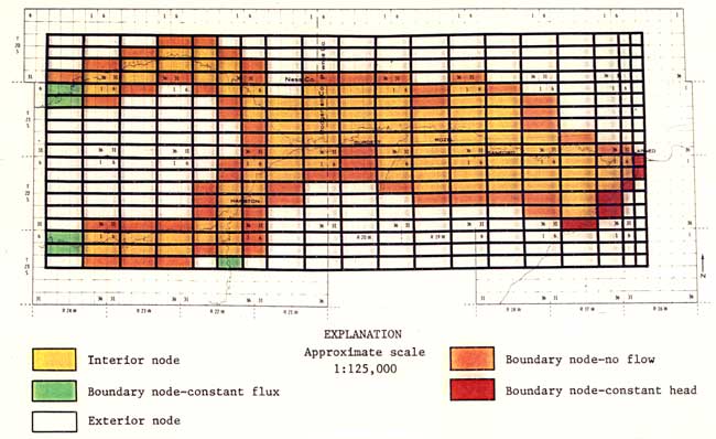
The 1945-47 water-level map of Pawnee Valley was employed to calculate the hydraulic gradients at the western and southwestern boundaries of the modeled aquifer (Fig. 26). The fluxes at these boundaries were calculated using Darcy's law, which in a simplified form may be expressed as
Q = K A I (6)
where, Q = amount of ground water entering the study area (L3 / T)
K = hydraulic conductivity of the aquifer material (L / T)
A = cross-sectional area through which flow takes place (L2)
and I = hydraulic head gradient or slope of the water-table (L / L)
The hydraulic conductivity used was the initial average value of hydraulic conductivity for the Pawnee Valley sediments derived from the pump tests described in Fishel (1952; see Part A of this report). The averaging procedure used for the hydraulic conductivity is the geometric mean.
[Note: The geometric mean G of a set of N numbers X1, X2, ..., XN is the Nth root of the product of the numbers:
The logarithm of the geometric mean is the mean of the logarithms of the individual values. The geometric mean of a set of positive numbers X1, X2, ..., XN is less than or equal to their arithmetic mean, but is greater than or equal to their harmonic mean. The equality holds only if all the numbers X1, X2, ..., XN are identical. Of the five pump tests described in Fishel (1952), the arithmetic mean is 472.2 ft/day, the geometric mean is 242.7 ft/day, and the harmonic mean is 152.6 ft/day.]
There is a large body of evidence (Freeze, 1975) to support the observation that the probability density function for hydraulic conductivity is log normal. In log normal distributions the appropriate average is the geometric mean, which has properties analogous to those of the arithmetic mean of a normal distribution.
Using the above data and the parameter adjustment routine built into the model (see further explanations under the section "Parameter estimation or model calibration"), the net groundwater fluxes entering the western boundaries of the model area were calculated to be approximately 650 acre-feet per year for the Ness-Hodgeman portion of the valley, and approximately 11,830 acre-feet per year for the valley portion west of Jetmore; the net groundwater flux entering the southwestern portion of the valley near the confluence of Saw Log Creek and Buckner Creek was found to be approximately 1,190 acre-feet per year. It should be noted that the net groundwater fluxes were calculated by subtracting from the boundary fluxes the amount of annual appropriated pumpage to the wells in the boundary grid subregions over which the fluxes were calculated. The high values of incoming fluxes in the Jetmore area, compared to the other boundary fluxes, suggest that groundwater contributions to the alluvial aquifer from the underlying Dakota aquifer are probable in that area.
These calculated boundary fluxes are kept constant throughout the predictive period employed in this report (20 years). This is a conservative assumption because, despite the water level declines and saturated-thickness reductions, the boundary fluxes are assumed constant.
The eastern boundary of the modeled area is the Arkansas River. This boundary is treated as a classical constant-head boundary that is time invariant. Such assumption is very conservative since the river becomes an unlimited source of water to the groundwater system as the water levels decline in the vicinity of the stream. This situation has led to the most optimistic forecasts for water levels in the region close to the Arkansas River; therefore, results should be viewed accordingly.
The bedrock and water-level data put into the model are described in the first part of this report. Initially uniform average values of hydraulic conductivity and storativity were used for all nodes. The average hydraulic conductivity used, using the averaging procedure described previously, was 2.04 acre-feet/ft2 while an assumed value for storativity (Fishel, 1952; see Part A of this report) of 0.15 was employed.
The values of the net pumpage required by the model for each node were determined as follows. First, all registered wells were inventoried from the records of the Kansas State Board of Agriculture, Division of Water Resources in Topeka and their field office in Stafford, as well as from Groundwater Management Districts No. 3 and No. 5. Special care was taken to check the location and appropriate pumpage of the wells by contacting the groundwater management districts' managers and checking questionable data at the Water Resources Division. In order to put all these wells into the model, the following procedure was used. All wells located within a grid subregion were assigned to the node at the center of the grid. In very few cases, if the grid was near a no-flow boundary and its average saturated thickness was very small, and that grid had one or more wells near the boundaries with a grid with higher saturated thickness, then the well or wells of that marginal grid were assigned to the nearest grid with a greater saturated thickness. This situation resulted from using one average value of saturated thickness and aquifer parameters for the entire grid subregion. Also, due to the relatively complex shape of the Pawnee Valley, the approximation of that geometry by the finite-difference grid resulted in some small parts of the Valley being located outside the model grid area. In that case, if wells existed in the part of the Valley near the grid boundary, they were assigned to the nearest grid node. The resulting distribution of the appropriated pumpage is indicated in Figure 27. Because the wells in the valley are not water-metered and the farmers' water-use reports are incomplete (not all irrigating farmers submit such reports), the pumpage data used in the model are the amounts appropriated by the Water Resources Division. In cases of overlapping water rights, it is assumed that all overlapping wells are pumping simultaneously over each period and that the amount they pump is the average value derived by dividing the maximum amount of pumpage assigned to the water right divided by the total number of overlapping wells. A complete listing of all registered wells in the alluvial aquifer and their appropriated pumpages in the Pawnee Valley portions of Pawnee, Hodgeman, and Ness counties is included in Appendix A.
Figure 27--Total amount of groundwater (in acre-feet) appropriated per year to wells in the area of each block.
The present computer model, however, operates on net pumpage values--that is, amounts of gross pumpage minus any amounts of irrigation return flow and natural recharge with no water gain or loss occurring through the base of the aquifer. Since it is assumed that approximately 10% of the amount of water pumped returns as deep percolation to the water table, all amounts of pumpage are adjusted accordingly (H. Dickey, 1979, oral communication). Also, as described in the first part of this report, the average natural recharge over the area is approximately 0.5 inches per year and all amounts of pumpage are adjusted accordingly.
Some model features designed for the Pawnee Valley
The computer program, as modified for the present study, determines if heads have fallen below the bottom of the aquifer. If so, those heads are set equal to the bottom elevation plus 0.01 foot. Thus, the aquifer transmissivity always has some positive value, allowing refilling of the aquifer if the opportunity ever occurs.
There are many alternatives available if a well runs dry, e.g., turning the pump off, reducing the pumpage to match the aquifer capabilities, shifting pumpage to other wells, or using some combination of these. There are a few empirically derived formulas relating the reduction of pumpage to the saturated thickness and other aquifer parameters (Lappala, 1978) but these relationships are for thick and relatively deep aquifers as opposed to the thin, shallow Pawnee Valley alluvial aquifer. Besides, no data were available to empirically derive a similar relationship for Pawnee Valley. For these reasons, as an option, it is conservatively and arbitrarily assumed that the wells are able to pump their original appropriation until the saturated thickness declines down to eight feet or less at which time the well is shut down; but the same well does not resume pumping until the saturated thickness is built up to 15 feet or more. Another option employed consists of allowing the well to deplete not more than 40% of the initial saturated thickness, at which time the well is shut down; the same well is assumed to resume pumping when the saturated thickness is built up to 62% or more of the original saturated thickness. Some further model modifications are discussed later in the section on projected water-level declines.
Prev Page--Hydrogeology, Hydrogeochemistry || Next Page--Calibration