PfEFFER Concepts Productivity

Productivity

Calculations of water saturation from either the Archie equations or the Pickett plot when combined with porosity gives values which describe the volume of water and hydrocarbon as a fraction of either pore space or the total rock. However, this knowledge is not sufficient in of itself to determine whether a zone will produce hydrocarbons, water, or hydrocarbon-cut water. Even if hydrocarbons are produced on test, will they prove to be economic? Although local rules-of-thumb are often quite satisfactory, there are numerous instances of zones with high water saturations that produce water-free hydrocarbons and others with low water saturations that produce high water cuts. The missing element to be considered is the relative size of the pore bodies and pore throats. In this section we will see how the bulk volume water (BVW) is a useful measure that is controlled by both pore size and possible position in the hydrocarbon column, and how this information can improve predictions concerning a zone's likely fluid productivity.

The idealized reservoir profile in Figure 10 shows the expected fluid production as a function of water saturation, porosity and height in a homogeneous petrofacies. The relationships reflect buoyancy pressure of the hydrocarbons that penetrate progressively smaller pore throats at greater column heights and a tendency for larger pore throats in higher porosity zones. High in the reservoir, the water saturations of zones will approach an “irreducible” water saturation that is determined by their pore geometry. Sometimes this saturation is called “immobile” or “ineffective”, because high-pressure laboratory tests show that these saturations are not absolutely irreducible. However, the “irreducible” water saturation generally marks a point at which hydrocarbons have permeated the entire macropore system and are subject to Darcian fluid flow and most of the remaining water is held either at grain surfaces or within micropores by capillary forces.

The plot of porosity against water saturation (Fig. 10) shows the hyperbolic trend at “irreducible” saturation that is typical of many reservoirs. The hyperbola is approximated by the function:

This general inverse relationship between irreducible water saturation and porosity that was noted by several early authors, including Archie (1952). They correctly attributed differences in the curvilinear trends to differences in reservoir pore sizes. This is because irreducible water saturation is controlled by surface tension at the internal surfaces and capillary pressure. While zones at irreducible water saturation in a moderately homogeneous reservoir should lie on a common curve, transition zones will be displaced to higher values of bulk water volume (F*Swi). The distinction is important, because it determines which zones should produce water-free oil or gas, and which should produce water or water-cut hydrocarbon. Computations of bulk volume water are therefore a critical additional step in log analysis for the assessment of producibility, as pointed out by Morris and Biggs (1967), Asquith (1985 ) and others.

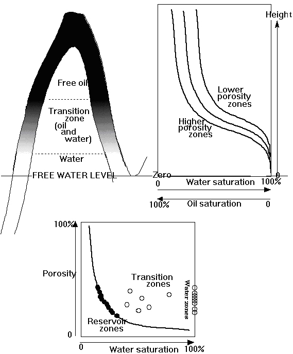Figure 10: Generalized reservoir profile with matched water saturation-height plot and porosity-water saturation crossplot.

Buckles (1965) made an extensive numerical analysis of reservoir measurements and concluded that the quadrilateral hyperbolic function: was a good first-order approximation to real field data. Low values of c reflected large average pore sizes, high values were linked with finer pores, as a direct consequence of a control by internal surface area. The critical hyperbolae that match different values of c can be drawn on a water saturation -porosity plot (often known as a “Buckles plot”) either on arithmetic scale or (less commonly) on a logarithmic scale (Figure 11). An advantage of the log scale format is that the hyperbolic curves plot as straight lines.

The quantity c, is simply the irreducible bulk volume water (BVWi) which will be effectively a constant, provided that there is a limited range in pore size. Zones with comparable pore size that have higher values of bulk water volume should be water-cut or totally water-bearing. When computed for a field or reservoir, the characteristic value is often known as the "Buckles number".

The zones from the hypothetical Rottweiler Sandstone example are plotted on these variants of the Buckles plot in Figure 11. If this was a real data set, then the hyperbolic trend of zones A-E, coupled with their low Buckles number of about 0.05, would be highly suggestive of zones at irreducible saturation. Water-free production would be expected for these zones, in contrast with Zone F which should produce mostly water with little or no hydrocarbons. (Obviously, no hydrocarbons would be expected from zones G-J.)

What are the values of c that should be expected for any given reservoir? The answer may be given either with respect to the type of reservoir rock or in terms of the values that have been reported from nearby fields that have produced from the same formation. So, for example, Asquith (1985) suggests rule-of-thumb numbers for carbonates keyed to pore type. Alternatively, expectations may be linked with geological formation, such as shown in the guide of critical BVWs reported by Bill Guy (Fig. 12), based on his extensive log analysis experience of Kansas fields.

Rather than tying our estimates to unique values of critical BVW, we can expand our consideration to ranges observed in field data. Reservoir values of c are shown plotted as cumulative frequency curves in the upper part of Figure 13 for carbonate reservoirs with vugular and intercrystalline/intergranular porosities (based on data from Chilingar et al, 1972 ) and for sandstones (using data from Bond, 1978 ). The data show systematic trends that reflect distinctions in internal surface area, and provide values that are useful in the following analysis. In the lower part of Figure 13, an example is shown of cumulative frequency curves plotted from data of well-known Texas carbonate reservoirs.

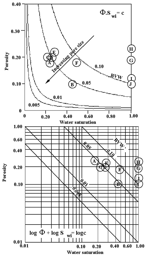Figure 11: Rottweiler Sandstone zones located on Buckles plots - arithmetically scaled (above); logarithmically scaled (below)

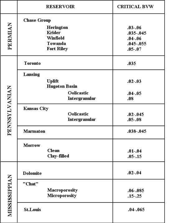Figure 12: Typical values of critical bulk volume water (or Buckles number) for reservoirs in Kansas. These "rules-of-thumb" ranges were developed on the basis of extensive field experience.

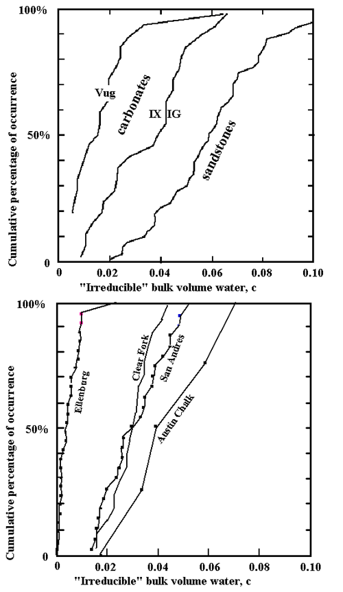Figure 13: Cumulative frequency plots of irreducible bulk volume water for reservoirs by pore type (above) and by Texas carbonate formation (below).

Plotting Bulk Volume Water (BVW) lines on the Pickett plot

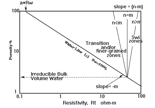
Pickett (1973) had recognized that reservoir zones at irreducible water saturation should tend to lie on a steeper linear trend, whose intercept with the water line reflected the grain- or pore-size. This observation reflects the fact that the hyperbolic relationship of :

can be linearized to :

Substituting the Archie equation solution for water saturation and rearranging, the relationship becomes :

which describes a line on the Pickett plot with a slope of (n-m) and an intersection with the water line at a porosity corresponding to the water line .

Greengold (1986) was the first to describe the systematic graphic properties of the irreducible bulk volume water on the Pickett plot. When the cementation and saturation exponents are equal, zones at irreducible water saturation should follow a line parallel to the porosity axis (Figure 14). Otherwise, the line will be inclined according to whether the saturation exponent is greater or less than the cementation exponent. Notice that any Buckles number line will intersect the water line at a porosity value equal to the Buckles number value. It will also cross the 100% porosity limit at a water saturation value equal to the Buckles number value.

The parameters that determine the line give a powerful new means to extend the function of the Pickett plot beyond its traditional roles of cementation exponent and formation water resistivity. If the irreducibly saturated zones form a coherent trend, then the saturation exponent can be estimated directly from the plot for water saturation calculations, while the producibility will be indicated for any zone.

Bulk volume water contour lines are plotted for the Rottweiler sandstone on the Pickett plot used earlier (Figure 15). As observed before, zones A to E tend to follow a Buckles number value of about 0.05. The linear trend reflects a matching hyperbolic trend if the zones were plotted in a linear porosity - water saturation scaled graph (as seen in Figure 11). In fact, this adaptation of the Pickett plot represents the incorporation of the “Buckles plot”.

Figure 14: Location of irreducible bulk volume water (Buckles number) trend on Pickett plot.

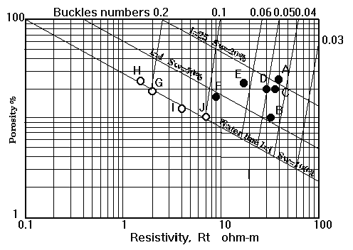Figure 15: Location of Buckles lines on the Pickett plot of Rottweiler Sandstone data.