![]()
Prev Page--Formations || Next Page--Hydrology
Ground Water
Role of Ground Water in the Water Cycle
Ground water is defined by Meinzer (1923) as that part of the subsurface water that is in the zone of saturation. The subsurface water above the zone of saturation--that is, water in the zone of aeration--is called suspended subsurface water or vadose water. Ground water takes a small but very important part in the water cycle.
Basically, ground water is derived from precipitation in the form of rain or snow. Part of the precipitation runs off directly into streams; a large part of the precipitation is absorbed by the soil, from which much of it evaporates directly or is absorbed by vegetation and later evaporated into the atmosphere. The rest percolates slowly downward through the soil and underlying strata until it reaches the water table, where it joins the body of ground water in the zone of saturation. This is the zone saturated with water under hydrostatic pressure.
Ground water percolates slowly through the rocks in directions determined by the geology, topography, and geologic structure until it is discharged eventually into surface-water bodies through springs and seeps, by withdrawal from wells, or by evaporation and transpiration in areas where the water table is shallow.
Movement of Ground Water
In Ottawa County, ground water moves toward the major streams; and, once it reaches the terrace deposits, it flows toward the streams but with a down-valley component. Thus, part of the ground water discharges into the river and becomes surface water. Ground water moves through the Dakota Formation into the north-central part of the county from Cloud County, and some enters the southwestern corner of the county from Saline and Lincoln counties; otherwise, most ground-water movement is away from Ottawa County. Large amounts of ground water move through the terrace deposits into the county in the Solomon and Saline River valleys. A smaller amount enters in Salt Creek valley.
More than 200 wells were inventoried for the preparation of a map showing the configuration of the piezometric surface (Pl. 7). This is the surface of the water table or the height to which water, under hydrostatic pressure, will rise in a well. This surface, roughly parallel to the topography, in Ottawa County, fluctuates as ground water is discharged or recharged. All points on each contour line on Plate 7 are at an equal altitude above sea level. A line crossing perpendicular to the contour lines indicates the direction of ground-water movement as it passes from a higher to a lower altitude. Because of the lack of water in the Wellington Formation, piezometric contours are not given in areas of outcrop of this formation.
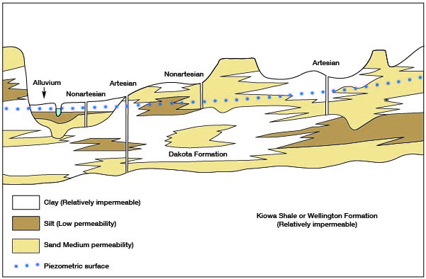
Many of the inventoried wells are in the Dakota Formation, which contains water under hydrostatic and atmospheric pressure (artesian) and water under atmospheric pressure only (nonartesian). The conditions under which the Dakota was deposited were such as to cause lenticularity of all beds. Thus, the Dakota Formation is composed of intertonguing lenses of permeable sand, less permeable silt, and relatively impermeable clay (Fig. 6).
Figure 6--Diagrammatic cross section of Dakota Formation and river terraces in Ottawa County showing intertonguing lenticular beds of different permeability, typical artesian and nonartesian wells, and hydraulic gradient.
Water-level records, chemical analysis of water, and geologic studies indicate an interconnected hydraulic system within the Dakota Formation. Some wells in the Dakota Formation obtain perched water from zones that lie above the piezometric surface. A few wells obtain water from a deep zone in the Dakota Formation in which the static water level is below the piezometric surface in nearby wells. The hydraulic connection between the zones is very poor or does not exist. Only 12 out of more than 300 test holes and inventoried wells obtained water from perched or deep zones.
Upper Pleistocene terrace deposits, although stratigraphically separated from the Dakota Formation, are hydraulically connected with it (Pl. 8). Terrace deposits are composed of stratified sediments that grade upward from coarse to fine material. Numerous test-hole samples show that, in many places, saturated sandstone of the Dakota Formation directly underlies basal sand and gravel in the terrace deposits. In addition, numerous massive sandstones of the Dakota adjoin the terrace borders. Static water-level measurements show that the piezometric surface passes smoothly from the Dakota into the terrace deposits (pl. 7). Water-quality data do not distinguish between a Dakota or terrace-deposit source, except for local anomalies. Base flow discharge of Solomon River at Niles is about twice the discharge at Beloit in Mitchell County. Records of discharge at these stations are published in the annual series of Water-Supply Papers by the U. S. Geological Survey. Hence, data prove hydraulic interconnection between the Dakota and the terrace deposits and discharge of ground water from the Dakota into the terrace deposits.
Ground-water Recharge
Precipitation accounts for most of the ground-water recharge in Ottawa County. If the average annual precipitation in the county is assumed to be 26.6 inches, the average in Minneapolis, then Ottawa County receives an average of 1.0 million acre-feet of precipitation per year. Only a small fraction of the precipitation becomes ground water. Most is either returned to the atmosphere by evapotranspiration or discharged by direct runoff. The average rate of evapotranspiration in Ottawa County is 24 inches per year (Foley, Smrha, and Metzler, 1955). Slightly more than half this amount is transpired (1.03 feet) and slightly less than half is evaporated (0.97 foot). If the average precipitation is 26.6 inches and the average evapotranspiration is 24 inches, then 2.6 inches becomes runoff, which is equivalent to about 100,000 acre-feet. Thus, the runoff of about 100,000 acre-feet represents water that flows directly from the surface into the rivers and water that recharges the ground-water reservoir and then seeps into the rivers as ground-water discharge. Stream-flow analyses indicate that about half the total runoff is ground-water discharge. Hence, an average of about 50,000 acre-feet of water each year recharges the ground-water reservoir, moves down a hydraulic gradient, and discharges into streams.
Some ground water moves into Ottawa County from Cloud County. A smaller amount moves into the southwestern corner of the county from Saline and Lincoln counties.
In 1957 the amount of ground-water recharge due to irrigation from surface water was negligible. All irrigated areas are near a river or stream. As ground water normally discharges into the river or stream, any recharge to ground water would soon be routed back to the surface water. No shallow aquifers in Ottawa County are recharged by irrigation water obtained from a deeper aquifer.
Ground-water Discharge
Ground water discharges into bodies of surface water, primarily rivers, and to a lesser degree lakes and ponds, even during periods of drought; Solomon River continued to flow during the prolonged 1952-57 drought. Ground water discharging, without the agency of man, upon the land or into a body of surface water, is known as a spring or seep. Owing to the abundance of saturated sandstone that crops out in Ottawa County, springs and seeps are common. If there were less vegetation to absorb ground water near zones of discharge, springs would be more obvious. Vegetation uses ground water whenever plant roots reach the zone of saturation or the capillary fringe just above the water table. If ground water or the capillary fringe is sufficiently near the surface, evaporation will take place. The last two types of ground-water discharge are known jointly as evapotranspiration. Surface water and vadose water supply most water for evapotranspiration. A considerable amount of ground water moves in the subsurface from Ottawa County to all adjacent counties. The only ground water not discharged by natural causes is that pumped from wells. All the municipalities and most of the farms obtain their water from wells. Most farm and stock wells yield only a few gallons per minute, but municipal and irrigation wells yield 100 to 600 gpm.
The total amount of water pumped from wells in Ottawa County during 1957, itemized in Table 4, was about 1,280 acre-feet.
Table 4--Use and amount of ground water pumped during 1957.
| Use | Gallons per day | Acre-feet per year |
|---|---|---|
| Public supply | 359,000 | 400 |
| Rural domestic supply | 168,000 | 190 |
| Stock | 450,000 (est.) | 500 |
| Industry | 144,000 (est.) | 160 |
| Irrigation | 27,000 (est.) | 30 |
| Total | 1,280 |
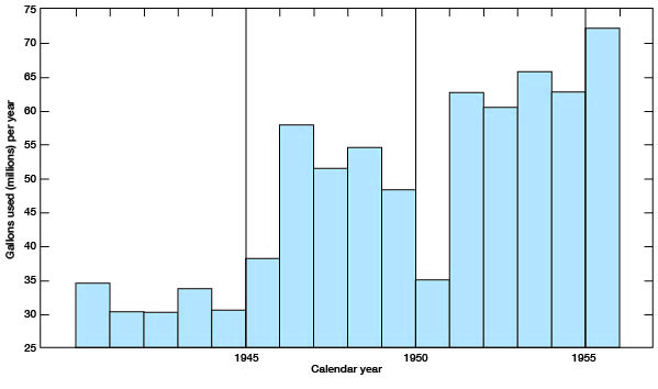
Although the population of Minneapolis has declined only slightly since the beginning of World War II, there has been a marked increase in the quantity of water used (Fig. 7). Throughout World War II, the consumption varied only slightly and ranged between 30 and 35 million gallons per year, or approximately 43 gallons per capita per day. Since World War II, with the exception of the 1951 flood year, the consumptive demand has increased greatly. In 1956, the quantity used was approximately 100 gallons per capita per day. Two main reasons account for this greater water consumption. There continues to be a large increase in appliances that require water; air conditioners, garbage-disposal units, lawn and garden sprinkling systems, and automatic washers are a few examples. In addition, many new household plumbing systems have been installed and old ones expanded. The other reason for increased water consumption was the drought from the fall of 1951 until the spring of 1957. Large quantities of water were used for gardens and lawns, and water was hauled from the city to rural areas.
Figure 7--Annual use of water at Minneapolis, 1941-1956.
Interrelations of Surface and Ground Waters
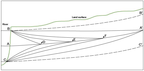
Normally, ground water is discharged into the rivers in Ottawa County. At times, however, the rivers lose water to the ground-water reservoir. Figure 8 shows a cross section of a river and adjoining water-table aquifer. It is assumed that the aquifer is homogeneous and isotropic (water flows with equal facility in any direction) and that there is no surface of seepage at the river bank. Under conditions of normal flow, water moves in dynamic equilibrium from source A' to the river level, A, in the direction of the hydraulic gradient A'A; ground water is being discharged into the river. If the river level should rise suddenly to B, then readjustment of the hydraulic gradient would commence immediately and pass consecutively through lines BDA', BEA', and BFA' until equilibrium was again regained along the hydraulic gradient A'B. A' has a slightly greater head than B, so the direction of flow would be toward the river again. During the readjustment of the hydraulic gradient there are simultaneously two slopes, BA and A'A, and hence, two directions of flow. When the river rises from A to B, the river recharges the ground-water reservoir, for example, along BD. But at this moment, water from the aquifer is still moving along A'D toward the river. At point D, the vector of flow is the resultant of BD and A'D vectors. In other words, at point D, the water level rises upward and slightly away from the river. When the hydraulic gradient is BEA', the curvilinear triangle BDE has become saturated by recharge from the river, and the vector at point E is almost vertical. By the time curvilinear triangle BEF is saturated, the vector at point F is upward and slightly toward the river. Water from the river is still recharging the groundwater reservoir but at a decreasing rate. Eventually the direction of flow will, at all points, be toward the river when equilibrium is regained between a pressure head at A' and a slightly lower point at B. The same principles are applied in reverse if the river is suddenly lowered from A to C. Steady-state conditions will be regained along A'C only after successive dewatering of curvilinear triangles CAD, CAE, CAF, and finally CAA'.
Figure 8--Effects of changes in stream level on adjacent water table.
In essence, a constant quantity of water flows in equilibrium along a constant gradient, according to Darcy's law, if the permeability, cross-sectional area, and difference in head are constant. But, if the head changes, along either a source or a drain, then two gradients form, which are connected by a point of flexure (or intermediate head) moving from the source or drain that was changed to the source or drain that remained unchanged until equilibrium is regained. The motion of the flexure point is the resultant vector of the gradient vectors.
River recharge to ground water in Ottawa County generally does not follow the above explanation except in areas where relatively homogeneous sandstone of the Dakota Formation is in contact with the river. Most of the valley fill is heterogeneous and includes several feet of silt and clay at the top. The piezometric surface in the valley fill is above the sand and gravel in many places. Numerous test holes show that it passes through silt and clay and that much of the ground water in the valleys is under slight artesian pressure. Under artesian conditions a rapid rise in the river level will not cause appreciable movement of water from the river toward the aquifer; but, instead, it will cause a rise in the piezometric surface. Because the piezometric surface outside the valley is higher than the top of the river bank, as shown by line AA' (Fig. 9), the water does not move into the aquifer. Theoretically, the rise of the piezometric surface should be instantaneous with a rise in the river level, but generally there is a time lag, increasing with distance away from the river because of elasticity of the valley fill and very slight compression of the water.
Figure 9--Diagrammatic cross section of typical river valley under artesian conditions. Relations between river stages and piezometric surface are shown.
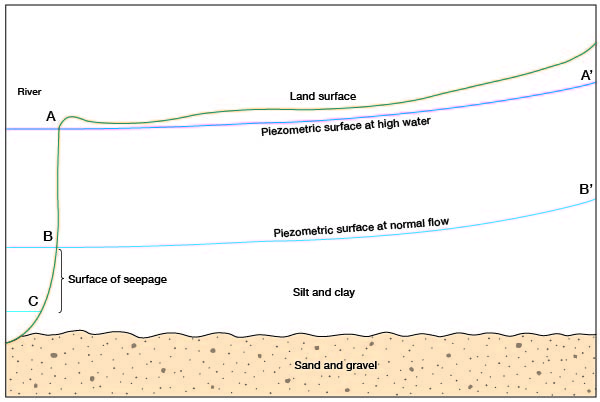
Along a gaining stream the piezometric surface is either level with or above the river stage if the aquifer and the river are connected hydraulically. Figure 9 shows, for example, the piezometric surface at BB' while the river stage could be either at B or at C. If the river stage is at C and the piezometric surface intersects the river bank at B, the distance between B and C is known as the surface of seepage. Commonly, it is the interface between flow in a porous medium and flow in an open channel. The surface of seepage occurs if water in the river can discharge at a rate greater than ground water can recharge it. Thus, by eliminating the surface of seepage, the rate of ground-water discharge to a stream can be determined if river discharge is controlled and measured (at a dam) so that the level of the river is equal in altitude to the piezometric surface. River discharge will equal increase in streamflow from ground-water discharge. This assumes, of course, that there is no evaporation or additional surface-water inflow. Ground-water discharge to the river may differ in amount from place to place, but the total quantity can be measured. If the total quantity of discharge is known, then the average permeability of the artesian aquifer can be determined by assuming a constant hydraulic gradient and area.
Ground-water discharge along the reach of a stream is generally assumed to equal the amount by which base flow increases through that reach. Base flow is the discharge of a stream without additional surface-water inflow. A surface of seepage, which may be as much as 10 feet wide in places along Solomon River, provides an ideal situation for evaporation. The potential rate of evaporation may exceed groundwater seepage, and the surface of seepage may seem dry. Because the piezometric surface is close to the land surface near the stream, the opportunity for transpiration by plants is great. Base flow, then, is equal to ground-water discharge minus an unknown but large amount of evaporation from the surface of seepage and transpiration by plants, under ordinary circumstances. If the rate of evaporation and transpiration exceeds the rate of ground-water discharge, the river will cease to flow.
Although the surface of seepage from an artesian aquifer is illustrated in the above example of determining ground-water discharge to a river, artesian conditions are not necessary. The surface of seepage is found wherever discharge from a drain (usually an open channel) exceeds recharge from a source having different flow rate or permeability (usually saturated material). It may be present under artesian or nonartesian conditions and in a two-dimensional (riverbank, dam) or a three-dimensional (well) hydraulic system.
Recharge of a Well by Surface Water
To understand the process by which a well is recharged by surface water, it is first necessary to understand the behavior of each hydraulic system. The last section discussed surface-water and ground-water systems, which were treated essentially as two-dimensional systems, the third dimension being regarded as infinite. The flow of water toward a well is radial, but lowering the water level (drawdown) by pumping creates a third dimension. Therefore, recharge to a well from a body of surface water is the addition of two-dimensional flow from surface water to the existing three-dimensional flow around a well.
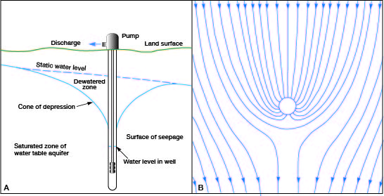
When a well in a water-table aquifer is pumped, the water level in the well is lowered, and water surrounding the well flows into it by the force of gravity. The surface of the water moving toward a well is that of a curvilinear cone having its vertex downward and is called the cone of depression. Its slope is controlled by the rate of discharge of the well, the permeability of the saturated material, and the thickness of the saturated material. Also, if the aquifer is not completely penetrated, the slope is affected. The cone of depression may be symmetrical or asymmetrical.
Ground water is in motion wherever there is a hydraulic gradient, as there is in nearly all natural ground-water reservoirs. When a well is pumped at a steady rate of discharge, an asymmetrical cone of depression will develop in the vicinity of the well (Fig. 10). When discharge ceases, the cone will disappear, and the water will approach the original static level. The process of filling the cone of depression takes exactly as long as forming it, assuming the hydraulic gradient to be the same. If the total discharge of all wells within a given ground-water reservoir is less than the recharge that maintains the hydraulic gradient, the ground-water reservoir will never be depleted. If the converse is true, then water is being mined, and the reservoir will be depleted. Recharge to ground water in Ottawa County far exceeds present discharge from wells.
Figure 1O--A, Diagrammatic cone of depression developed in nonartesian aquifer by pumping well. B, Plan view of flow lines in vicinity of pumping well.
The slope of the cone of depression formed by pumping a well is of the same nature as the slope of the surface of water draining from a body of surface water (river) into permeable material (Fig. 11). The lower two drawings in Figure 11 are plotted on a logarithmic scale horizontally for ease in visualization. In basic form,
Q = PIA
where Q is discharge, P is the coefficient of permeability, I is the slope or change in head per unit length, and A is the cross-sectional area.
Figure 11--A, Cross sections showing half cones of depression around well discharging water from nonartesian aquifer. B, River recharging dewatered permeable material. Each drawing shows three stages of equilibrium.
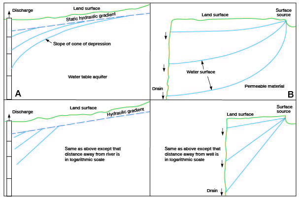
Thus, if water is being discharged from a well or draining into the ground-water reservoir from a river at the same rate (Q) in equilibrium, through porous material of identical permeability (P), and the area (A) along the river is chosen to equal the area around the well, the slopes (I) would be identical whether the river and well were hydraulically connected or completely separated. The flow capability through porous material is the same. Only the flow pattern toward a well or away from a river differs.
Aquifer Tests
Haddock Test
An aquifer test was made October 14, 1958, using an irrigation well owned by R. A. Haddock in the SE SE NW,14 sec. 21, T. 11 S., R. 3 W. The well has a diameter of 18 inches and a depth of 56.0 feet and is equipped with a turbine pump driven by a propane engine. The well yields water from Illinoisan terrace deposits. The static water level in the well prior to the test was 17.36 feet below the measuring point, which was 0.2 foot above land surface. Five observation wells were augered along a line S 45° E from the pumped well.
Table 5 is a summary of data on location and depth of wells used in this aquifer test; Table 6 gives the depths to water level measured during the test.
Table 5--Data on wells used in Haddock aquifer test.
| Well | Altitude of measuring point, feet | Height of measuring point above land surface, feet | Depth of well below measuring point, feet | Distance from pumped well, feet |
|---|---|---|---|---|
| Pumped well | 1,233.7 | 0.2 | 56.0 | |
| SE 1 | 1,233.0 | 0.0 | 31.3 | 10 |
| SE 2 | 1,235.4 | 2.4 | 40.8 | 50 |
| SE 3 | 1,235.9 | 3.0 | 38.4 | 100 |
| SE 4 | 1,235.5 | 2.4 | 37.4 | 150 |
| SE 5 | 1,235.9 | 3.0 | 35.1 | 300 |
Table 6--Depths to water measured during Haddock aquifer test.
| Pumped well |
Observation well SE 1 |
Observation well SE 2 |
Observation well SE 3 |
Observation well SE 4 |
Observation well SE 5 |
||||||
|---|---|---|---|---|---|---|---|---|---|---|---|
| Time since pumping began, minutes |
Depth to water from measuring point, feet |
Time since pumping began, minutes |
Depth to water from measuring point, feet |
Time since pumping began, minutes |
Depth to water from measuring point, feet |
Time since pumping began, minutes |
Depth to water from measuring point, feet |
Time since pumping began, minutes |
Depth to water from measuring point, feet |
Time since pumping began, minutes |
Depth to water from measuring point, feet |
| Static | 17.36 | Static | 16.64 | Static | 18.85 | Static | 19.37 | Static | 18.87 | Static | 19.46 |
| 4 | 39.43 | 5 | 19.03 | 6 | 26.04 | 9 | 20.23 | 8 | 19.25 | 8 | 19.74 |
| 7 | 41.80 | 9 | 20.33 | 11 | 27.10 | 13 | 20.69 | 14 | 19.81 | 10 | 19.96 |
| 11 | 42.50 | 12 | 21.01 | 19 | 27.66 | 17 | 21.15 | 22 | 20.30 | 12 | 20.13 |
| 23 | 39.60 | 15 | 21.35 | 25 | 27.78 | 20 | 21.60 | 28 | 20.60 | 14 | 20.30 |
| 27 | 40.05 | 19 | 21.66 | 31 | 27.90 | 23 | 21.87 | 33 | 20.80 | 16 | 20.47 |
| 31 | 39.30 | 21 | 21.80 | 36 | 28.02 | 26 | 22.17 | 39 | 20.96 | 18 | 20.63 |
| 36 | 39.12 | 24 | 22.06 | 42 | 28.08 | 29 | 22.31 | 45 | 21.10 | 20 | 20.78 |
| 42 | 39.30 | 29 | 22.27 | 48 | 28.14 | 32 | 22.56 | 51 | 21.20 | 22 | 20.90 |
| 46 | 39.60 | 34 | 22.47 | 54 | 28.20 | 35 | 22.74 | 57 | 21.25 | 24 | 21.02 |
| 52 | 39.80 | 39 | 22.68 | 67 | 28.30 | 38 | 22.90 | 70 | 21.38 | 26 | 21.12 |
| 56 | 39.83 | 44 | 22.85 | 75 | 28.38 | 41 | 23.05 | 80 | 21.45 | 28 | 21.23 |
| 61 | 39.87 | 49 | 22.95 | 85 | 28.43 | 44 | 23.17 | 98 | 21.55 | 30 | 21.34 |
| 67 | 39.61 | 54 | 23.09 | 95 | 28.50 | 46 | 23.28 | 114 | 21.62 | 34 | 21.43 |
| 72 | 38.85 | 59 | 23.21 | 103 | 28.53 | 49 | 23.38 | 126 | 21.63 | 36 | 21.50 |
| 76 | 39.55 | 64 | 23.31 | 123 | 28.60 | 52 | 23.47 | 138 | 21.72 | 39 | 21.60 |
| 81 | 39.88 | 69 | 23.40 | 136 | 28.66 | 55 | 23.54 | 153 | 21.79 | 44 | 21.70 |
| 86 | 40.35 | 74 | 23.43 | 151 | 28.70 | 61 | 23.69 | 169 | 21.85 | 49 | 21.79 |
| 96 | 40.85 | 79 | 23.57 | 167 | 28.76 | 68 | 23.82 | 189 | 21.92 | 54 | 21.86 |
| 106 | 39.52 | 84 | 23.65 | 187 | 28.82 | 73 | 23.91 | 209 | 21.98 | 59 | 21.93 |
| 122 | 40.14 | 94 | 23.79 | 207 | 28.87 | 79 | 23.98 | 228 | 22.08 | 64 | 21.99 |
| 134 | 39.30(?) | 104 | '23.93 | 226 | 28.91 | 83 | 24.04 | 248 | 22.13 | 69 | 22.05 |
| 149 | 40.35 | 121 | 24.16 | 246 | 28.95 | 96 | 24.18 | 268 | 22.19 | 74 | 22.08 |
| 164 | 40.10 | 135 | 24.39 | 266 | 29.02 | 101 | 24.22 | 79 | 22.12 | ||
| 184 | 39.85(?) | 150 | 24.54 | 110 | 24.29 | 94 | 22.16 | ||||
| 204 | 40.54 | 165 | 24.71 | 125 | 24.41 | 89 | 22.20 | ||||
| 224 | 39.60 | 186 | 24.85 | 137 | 24.47 | 94 | 22.26 | ||||
| 244 | 39.20(?) | 206 | 25.02 | 152 | 24.59 | 109 | 22.30 | ||||
| 264 | 40.10 | 225 | 25.17 | 168 | 24.68 | 119 | 22.34 | ||||
| 245 | 25.29 | 188 | 24.75 | 127 | 22.39 | ||||||
| 265 | 25.40 | 208 | 24.85 | 139 | 22.43 | ||||||
| 227 | 24.94 | 154 | 22.43 | ||||||||
| 247 | 25.00 | 170 | 22.54 | ||||||||
| 267 | 25.08 | 190 | 22.58 | ||||||||
| 210 | 22.64 | ||||||||||
| 229 | 22.69 | ||||||||||
| 249 | 22.72 | ||||||||||
| 269 | 22.76 | ||||||||||
The purpose of an aquifer test is to determine the hydraulic characteristics of an aquifer, from which optimum well spacing and pumping rates may be determined. Geologic and hydrologic factors affect the data from this test to a degree that mathematical treatment is not precise; nonetheless, a reasonable estimate of aquifer characteristics may be obtained.
Cooper and Jacob (1946) have shown that as time of pumping increases sufficiently, on semilogarithmic paper the plot of drawdown at a given observation well versus time approximates a straight line. If a period of time is chosen equal to a log cycle on logarithmic paper, then the equation reduces to
T = 264 Q / Δ s
where T is the transmissibility in gallons per day per foot throughout a 1-foot-wide strip extending the height of the saturated thickness of the aquifer, Q is the rate of discharge from the pumped well in gallons per minute, and Δ s is the drawdown, in feet, per logarithmic cycle.
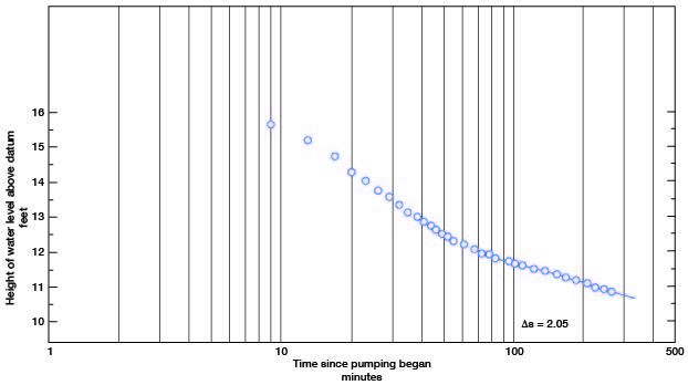
Figure 12 shows drawdown on the linear scale plotted against time on the logarithmic scale for observation well SE 3, which was 100 feet from the pumped well. Two gradients are seen. The steeper gradient is the drawdown under artesian conditions. After 4 feet of drawdown under artesian conditions, the gradient becomes more gentle. The log of the test hole shows about 4 feet of silt and clay below the static water level and 34.5 feet of sand and gravel beneath the silt and clay. Consequently, nonartesian conditions began to prevail as soon as the sand in the cone of depression started to become dewatered. If the pumping test were continued much longer at the same discharge, the slope would steepen very slowly, because of dewatering, until movement of water down the hydraulic gradient would cause the slope to flatten out, or the hydrologic boundary created by the valley wall would cause it to steepen more rapidly. Thus, it is reasonable to believe that the more gentle gradient in Figure 12 is the most suitable for determining the coefficient of transmissibility, because the effects of dewatering seemingly are not appreciable. Under the conditions where Q = 475 gpm and Δ s = 2.05,
T = (264)(475) / 2.05 = 61,000 gpd per foot.
As the transmissibility, T, is equal to the permeability, P, multiplied by the thickness of the saturated material, 34.5 feet, then P, in Meinzer units, equals 1,800 gpd per square foot under a hydraulic gradient of 100 percent at 60° F. The temperature of water during the test varied only between 58° and 58.5° F. The coefficient of storage, S, of an aquifer is defined as the volume of water released from or taken into storage per unit surface area of the aquifer per unit change in the component of head normal to that surface. Reasonableness of any estimate of the coefficient of storage might be questioned, owing to wide variation in the porosity and permeability throughout the aquifer and the change from artesian to nonartesion conditions.
Figure 12--Drawdown curve of observation well SE 3 during Haddock aquifer test. Datum is 1,200 feet above sea level.
Delphos Test
The Delphos test was made August 12, 1958, using the city of Delphos municipal well in the SE SW NW sec. 10, T. 9 S., R. 4 W. The well yields water from Illinoisan terrace deposits. It is 56 feet deep and is equipped with a turbine pump driven by an electric motor. Prior to the test, the static water level in the well was 37.03 feet below the base of the pump, which is 1.5 feet above land surface. Five observation wells were augered in a line N 40° W from the pumped well. Between observation well NW 1 and observation well NW 5, which are 10 and 300 feet respectively, from the pumped well, the thickness of sand decreases by 10 feet. Table 7 gives a summary of data on the wells used in this aquifer test. Table 8 contains the depths to water measured in each observation well during the Delphos aquifer test.
Table 7--Data on wells used in Delphos aquifer test.
| Well | Altitude of measuring point, feet | Height of measuring point above land surface, feet | Depth of well below measuring point, feet | Distance from pumped well, feet |
|---|---|---|---|---|
| Pumped well | 1,324.9 | 1.5 | 56 | |
| NW 1 | 1,325.2 | 2.3 | 55 | 10 |
| NW 2 | 1,324.9 | 3.7 | 53.8 | 50 |
| NW 3 | 1,321.5 | 0.2 | 44.5 | lot |
| NW 4 | 1,323.2 | 1.8 | 45.5 | 151 |
| NW 5 | 1,323.2 | 1.2 | 43.9 | 301 |
Table 8--Depths to water measured during Delphos aquifer test.
| Observation well NW 1 |
Observation well NW 2 |
Observation well NW 3 |
Observation well NW 4 |
Observation well NW 5 |
|||||
|---|---|---|---|---|---|---|---|---|---|
| Time since pumping began, minutes |
Depth to water from measuring point, feet |
Time since pumping began, minutes |
Depth to water from measuring point, feet |
Time since pumping began, minutes |
Depth to water from measuring point, feet |
Time since pumping began, minutes |
Depth to water from measuring point, feet |
Time since pumping began, minutes |
Depth to water from measuring point, feet |
| Static | 37.8 | Static | 37.6 | Static | 38.8 | Static | 39.0 | Static | 40.7 |
| 2 | 41.0 | 5 | 38.6 | 1 | 38.0 | 2.5 | 38.8 | 21 | 37.7 |
| 7 | 41.0 | 8 | 38.6 | 3 | 37.8 | 5 | 38.7 | 26 | 37.8 |
| 10 | 41.0 | 12 | 38.7 | 6 | 37.9 | 7.5 | 38.6 | 31 | 37.6 |
| 13 | 41.1 | 15 | 38.7 | 10 | 37.8 | 11 | 38.5 | 32 | 37.5 |
| 17 | 41.1 | 19 | 38.7 | 13 | 37.8 | 15 | 38.4 | 36 | 37.3 |
| 20 | 41.2 | 23 | 38.7 | 17 | 37.7 | 20 | 38.3 | 41 | 37.2 |
| 25 | 41.2 | 26 | 38.8 | 21 | 37.6 | 23 | 38.2 | 51 | 37.0 |
| 28 | 41.3 | 29 | 38.8 | 26 | 37.6 | 27 | 38.1 | 61 | 37.0 |
| 32 | 41.2 | 33 | 38.8 | 28 | 37.5 | 30 | 38.1 | 66 | 36.8 |
| 35 | 41.3 | 37 | 38.8 | 32 | 37.4 | 34 | 38.0 | 71 | 36.7 |
| 40 | 41.4 | 43 | 38.8 | 36 | 37.4 | 38 | 37.9 | 76 | 36.7 |
| 45 | 41.4 | 47 | 38.9 | 42 | 37.2 | 44 | 37.7 | 81 | 36.7 |
| 49 | 41.4 | 54 | 38.9 | 47 | 37.2 | 49 | 37.6 | 86 | 36.6 |
| 52 | 41.4 | 61 | 38.9 | 52 | 37.1 | 53 | 37.5 | 96 | 36.5 |
| 58 | 41.4 | 65 | 38.9 | 54 | 37.0 | 59 | 37.5 | 106 | 36.5 |
| 62 | 41.5 | 81 | 39.0 | 66 | 36.9 | 68 | 37.3 | ill | 36.3 |
| 79 | 41.6 | 87 | 39.0 | 81 | 36.6 | 83 | 37.1 | 123 | 36.2 |
| 83 | 41.6 | 95 | 39.0 | 91 | 36.6 | 92 | 37.0 | 138 | 36.1 |
| 93 | 41.6 | 100 | 39.1 | 93 | 36.5 | 95 | 37.0 | 153 | 36.0 |
| 98 | 41.7 | 119 | 39.1 | 97 | 36.5 | 100 | 36.9 | 169 | 36.0 |
| 118 | 41.7 | 134 | 39.2 | 107 | 36.4 | 109 | 36.8 | 187 | 36.0 |
| 133 | 41.8 | 150 | 39.2 | 120 | 36.3 | 122 | 36.8 | 199 | 35.9 |
| 149 | 41.8 | 165 | 39.3 | 135 | 36.2 | 136 | 36.7 | 216 | 35.9 |
| 164 | 41.9 | 182 | 39.3 | 151 | 36.1 | 152 | 36.6 | 230 | 35.8 |
| 180 | 42.0 | 195 | 39.3 | 166 | 36.0 | 168 | 36.5 | 244 | 35.8 |
| 194 | 41.9 | 210 | 39.3 | 184 | 35.9 | 185 | 36.4 | 258 | 35.8 |
| 209 | 41.9 | 226 | 39.3 | 196 | 35.8 | 197 | 36.4 | 274 | 35.8 |
| 225 | 41.9 | 240 | 39.4 | 211 | 35.7 | 213 | 36.4 | 288 | 35.8 |
| 239 | 41.9 | 254 | 39.4 | 227 | 35.6 | 229 | 36.4 | 304 | 35.8 |
| 253 | 41.9 | 270 | 39.4 | 241 | 35.6 | 242 | 36.3 | 319 | 35.8 |
| 269 | 41.9 | 284 | 39.4 | 255 | 35.5 | 257 | 36.3 | ||
| 283 | 42.0 | 300 | 39.5 | 271 | 35.5 | 272 | 36.3 | ||
| 299 | 42.0 | 315 | 39.5 | 285 | 35.5 | 287 | 36.3 | ||
| 314 | 42.0 | 301 | 35.4 | 303 | 36.3 | ||||
| 316 | 35.4 | 318 | 36.3 | ||||||
The municipal well was shut off for 20 hours prior to the aquifer test so that the water level could recover. Water levels in the observation wells were measured just before the test was to begin and it was found that water levels in the two observation wells nearest the supply well were still rising, and water levels in the other three observation wells were declining. An analysis of the data shows that NW 1 and NW 2 were fully penetrating wells and that the rising water was filling the dewatered sand under nonartesian conditions. Wells NW 3, NW 4, and NW 5, however, were not fully penetrating, because of caving. The aquifer thins in their direction. These three wells probably were outside of the dewatered zone and in the area of slight natural artesian pressure, but the bases of the wells were in materials of less permeability in the upper part of the aquifer, and hence the water levels measured in the wells were not indicative of the true piezometric surface. The aquifer test seems to support this explanation. The water levels in wells NW 1 and NW 2 declined rapidly at first but soon steadied to a very slow decline. Water levels in observation wells NW 3, NW 4, and NW 5 continued to rise throughout the test but were nearing equilibrium at the end of the test. The plot of water levels on a distance-drawdown graph on semilogarithmic paper formed a nearly straight line (Fig. 13) through values obtained near the end of the test, hence, pre-pumping water-level anomalies had disappeared, and inasmuch as the water levels were scarcely changing, the entire well system was nearing equilibrium. When water levels were measured the next day, there was no appreciable change in the cone of depression under pumping. It would seem, therefore, that the well under pumping has a large cone of depression around it approaching equilibrium when the pump is operating, and diminishing only slightly when the pump automatically stops for short periods. In addition, under normal automatic pump operation the piezometric surface transcends the nonartesian-artesian boundary.
Figure 13--Profile of cone of depression during Delphos aquifer test. Datum is 1,200 feet above sea level.
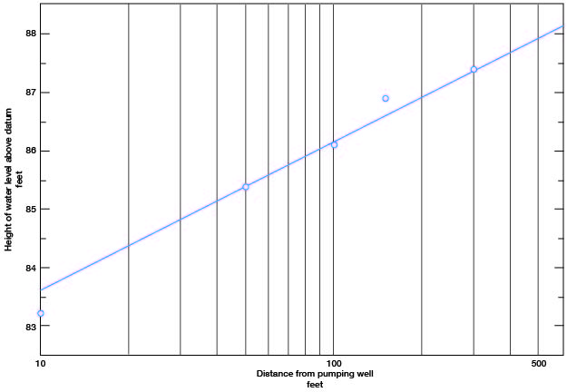
An equilibrium equation by Thiem (1906) has been transformed into convenient units by Wenzel (1942, p. 81) where
Pf = [527.7 Q log10(r2/r1)] / [m(s1 - s2)]
Pf is the coefficient of permeability at the prevailing water temperature, Q is the discharge in gallons per minute, m is the average saturated thickness, in feet, between observation wells, and s1 and s2 are the drawdowns, in feet, in observation wells at distances of r1 and r2 from the pumped well. When Q = 250, m = 14.4, s1 = 2.6, s2 = 0.6, r1 = 50, and r2 = 300, then
Pf = [527.7 250 log10(300/50)] / [14.4)(2)] = 3,570
T = Pf m = (3,570) (14.4) = 51,000 gpd/ft.
An easier solution is made by plotting drawdown, s, linearly and distance, r, logarithmically on semilogarithmic paper (Fig. 13). If permeability, Pf, and thickness, m, are replaced by transmissibility, T, then the equation becomes
T = (528 Q) / Δs
where Δs is the change in drawdown per log cycle of distance, r.
T = (528) (250) / 2.6 = 51,000 gpd/ft.
These equations are valid only if the cone of depression is in approximate equilibrium. As aquifer-test data show that the cone of depression was not appreciably altered in shape or size, the coefficients of permeability and transmissibility are believed to be fairly accurate.
State Lake Test
An aquifer test was made August 6-8, 1958, at the site of a public supply well in a recreation area in the NW NW SE sec. 8, T. 11 S., R. 2 W., 200 feet east of Ottawa County State Lake. The well has a diameter of 6 inches and a depth of 48.2 feet and yields water from the Dakota Formation. Prior to the test, the static water level was 17.80 feet below the top of the casing, which is 0.2 foot above land surface. Fifteen observation wells were augered in lines west, northwest, north, and east from the pumped well. All wells penetrate a thick, fine- to medium-grained, well-sorted, poorly consolidated quartzose sandstone extending from the surface to an undetermined depth below the wells. Observation well W 2 seemed to be partly plugged throughout the test. Otherwise the correct level of the nonartesian piezometric surface was observed in all observation wells.
Table 9 is a summary of data on the wells used in this test. Table 10 gives the depths to water level during the aquifer test.
Table 9--Data on wells used in State Lake aquifer test.
| Well | Altitude of measuring point, feet | Height of measuring point above land surface, feet | Depth of well below measuring point, feet | Distance from pumped well, feet |
|---|---|---|---|---|
| Pumped well | 1,311.8 | 0.2 | 48.7 | 0 |
| W 1 | 1,311.4 | 2.5 | 35.7 | 40 |
| W 2 | 1,309.8 | 2.4 | 31.3 | 80 |
| W 3 | 1,305.2 | 1.0 | 24.4 | 120 |
| W 4 | 1,302.1 | 3.5 | 17.5 | 160 |
| W 5 | 1,299.8 | 2.5 | 14.2 | 180 |
| W 6 | 1,297.8 | 2.0 | 11.2 | 195 |
| W 7 | 1,296.8 | 1.0 | 13.8 | 199 |
| Lake | 1,294.0 | 0 | 0 | 202 |
| NW 1 | 1,307.1 | 0.6 | 30.5 | 60 |
| NW 2 | 1,303.8 | 1.6 | 21.5 | 121 |
| N 1 | 1,307.8 | 0.4 | 23.0 | 40 |
| N 2 | 1,306.8 | 2.4 | 18.3 | 140 |
| N 3 | 1,302.9 | 1.8 | 18.5 | 181 |
| N 4 | 1,300.0 | 1.9 | 13.7 | 221 |
| E 1 | 1,320.8 | 4.0 | 45.7 | 100 |
| E 2 | 1,320.8 | 4.0 | 40.7 | 200 |
Table 10--Depths to water level measured during State Lake aquifer test.
| Observation well W 1 |
Observation well W 2 |
Observation well W 3 |
Observation well W 4 |
Observation well W 5 |
|||||
|---|---|---|---|---|---|---|---|---|---|
| Time since pumping began, minutes |
Depth to water from measuring point, feet |
Time since pumping began, minutes |
Depth to water from measuring point, feet |
Time since pumping began, minutes |
Depth to water from measuring point, feet |
Time since pumping began, minutes |
Depth to water from measuring point, feet |
Time since pumping began, minutes |
Depth to water from measuring point, feet |
| Static | 17.76 | Static | 16.78 | Static | 11.59 | Static | 8.44 | Static | 6.07 |
| 57 | 18.67 | 58 | 17.04 | 59 | 11.70 | 60 | 8.45 | 61 | 6.06 |
| 120 | 18.93 | 121 | 17.11 | 122 | 11.80 | 126 | 8.54 | 128 | 6.17 |
| 173 | 18.99 | 175 | 17.25 | 176 | 11.84 | 177 | 8.52 | 178 | 6.18 |
| 243 | 19.07 | 244 | 17.36 | 245 | 11.90 | 246 | 8.57 | 247 | 6.19 |
| 296 | 19.10 | 297 | 17.37 | 298 | 11.90 | 299 | 8.56 | 300 | 6.23 |
| 359 | 19.11 | 360 | 17.37 | 361 | 11.88 | 362 | 8.59 | 363 | 6.24 |
| 416 | 19.13 | 417 | 17.38 | 418 | 11.92 | 419 | 8.60 | 419 | 6.27 |
| 478 | 19.21 | 479 | 17.46 | 480 | 11.91 | 481 | 8.77 | 482 | 6.34 |
| 533 | 19.23 | 535 | 17.49 | 536 | 11.92 | 538 | 8.70 | 539 | 6.35 |
| 593 | 19.22 | 594 | 17.50 | 596 | 12.04 | 598 | 8.69 | 599 | 6.34 |
| 658 | 19.23 | 659 | 17.49 | 660 | 12.04 | 661 | 8.71 | 662 | 6.32 |
| 720 | 19.36 | 721 | 17.55 | 722 | 12.05 | 724 | 8.71 | 725 | 6.32 |
| 779 | 19.43 | 783 | 17.57 | 785 | 12.10 | 789 | 8.72 | 794 | 6.32 |
| 896 | 19.44 | 900 | 17.62 | 903 | 12.11 | 925 | 8.73 | 926 | 6.31 |
| 1,022 | 19.51 | 1,026 | 17.66 | 1,027 | 12.14 | 1,052 | 8.74 | 1,055 | 6.32 |
| 1,184 | 20.03 | 1,187 | 17.87 | 1,191 | 12.24 | 1,194 | 8.78 | 1,195 | 6.35 |
| 1,259 | 20.26 | 1,261 | 17.95 | 1,263 | 12.29 | 1,264 | 8.78 | 1,266 | 6.35 |
| 1,310 | 20.31 | 1,311 | 18.00 | 1,313 | 12.32 | 1,315 | 8.80 | 1,316 | 6.39 |
| 1,425 | 20.40 | 1,426 | 18.10 | 1,427 | 12.38 | 1,428 | 8.85 | 1,429 | 6.43 |
| 1,543 | 20.42 | 1,544 | 18.11 | 1,545 | 12.40 | 1,546 | 8.88 | 1,547 | 6.46 |
| 1,669 | 20.63 | 1,670 | 18.23 | 1,671 | 12.47 | 1,672 | 8.93 | 1,673 | 6.47 |
| 1,790 | 20.60 | 1,791 | 18.28 | 1,792 | 12.48 | 1,793 | 8.95 | 1,793 | 6.47 |
| 1,906 | 20.65 | 1,907 | 18.30 | 1,908 | 12.53 | 1,909 | 8.96 | 1,910 | 6.56 |
| 2,028 | 20.57 | 2,029 | 18.33 | 2,030 | 12.56 | 2,031 | 9.03 | 2,032 | 6.60 |
| 2,138 | 20.70 | 2,140 | 18.39 | 2,143 | 12.61 | 2,145 | 9.05 | 2,148 | 6.60 |
| 2,332 | 20.63 | 2,335 | 18.41 | 2,339 | 12.66 | 2,341 | 9.08 | 2,345 | 6.63 |
| 2,454 | 20.64 | 2,456 | 18.44 | 2,460 | 12.67 | 2,461 | 9.10 | 2,464 | 6.64 |
| 2,575 | 20.63 | 2,578 | 18.45 | 2,581 | 12.68 | 2,583 | 9.10 | 2,586 | 6.66 |
| 2,727 | 20.60 | 2,728 | 18.46 | 2,729 | 12.71 | 2,731 | 9.12 | 2,732 | 6.65 |
| 2,810 | 20.60 | 2,811 | 18.47 | 2,812 | 12.71 | 2,813 | 9.11 | 2,813 | 6.67 |
| Observation well W 6 |
Observation well W 7 |
Observation well NW 1 |
Observation well NW 2 |
Observation well N 1 |
|||||
|---|---|---|---|---|---|---|---|---|---|
| Time since pumping began, minutes |
Depth to water from measuring point, feet |
Time since pumping began, minutes |
Depth to water from measuring point, feet |
Time since pumping began, minutes |
Depth to water from measuring point, feet |
Time since pumping began, minutes |
Depth to water from measuring point, feet |
Time since pumping began, minutes |
Depth to water from measuring point, feet |
| Static | 4.10 | Static | 3.10 | Static | 13.70 | Static | 10.28 | Static | 14.15 |
| 62 | 4.13 | 63 | 3.19 | 66 | 13.93 | 65 | 10.30 | 72 | 15.07 |
| 129 | 4.15 | 130 | 3.19 | 133 | 14.13 | 132 | 10.32 | 138 | 15.34 |
| 179 | 4.15 | 180 | 3.20 | 183 | 14.27 | 181 | 10.36 | 184 | 15.42 |
| 248 | 4.21 | 249 | 3.25 | 253 | 14.40 | 251 | 10.40 | 257 | 15.50 |
| 300 | 4.22 | 301 | 3.27 | 303 | 14.47 | 302 | 10.45 | 308 | 15.53 |
| 363 | 4.25 | 364 | 3.27 | 366 | 14.50 | 365 | 10.47 | 371 | 15.54 |
| 420 | 4.24 | 421 | 3.:30 | 423 | 14.55 | 423 | 10.49 | 428 | 15.57 |
| 483 | 4.35 | 483 | 3.38 | 485 | 14.64 | 484 | 10.56 | 486 | 15.66 |
| 540 | 4.35 | 541 | 3.39 | 548 | 14.66 | 558 | 10.61 | 545 | 15.66 |
| 600 | 4.37 | 601 | 3.38 | 603 | 14.68 | 604 | 10.59 | 606 | 15.66 |
| 663 | 4.33 | 663 | 3.35 | 665 | 14.70 | 665 | 10.60 | 667 | 15.69 |
| 726 | 4.32 | 727 | 3.34 | 730 | 14.76 | 729 | 10.61 | 732 | 15.78 |
| 797 | 4.32 | 801 | 3.36 | 806 | 14.80 | 811 | 10.65 | 813 | 15.89 |
| 929 | 4.31 | 931 | 3.37 | 907 | 14.84 | 910 | 10.67 | 91.1 | 15.91 |
| 1,058 | 4.32 | 1,060 | 3.37 | 1,031 | 14.90 | 1,033 | 10.68 | 1,036 | 15.97 |
| 1,200 | 4.35 | 1,202 | 3.39 | 1,208 | 15.16 | 1,205 | 10.77 | 1,211 | 16.55 |
| 1,267 | 4.36 | 1,269 | 3.46 | 1,273 | 15.29 | 1,271 | 10.81 | 1,275 | 16.72 |
| 1,317 | 4.37 | 1,318 | 3.47 | 1,329 | 15.37 | 1,327 | 10.84 | 1,330 | 16.81 |
| 1,430 | 4.42 | 1,431 | 3.47 | 1,433 | 15.52 | 1,432 | 10.89 | 1,433 | 16.90 |
| 1,548 | 4.42 | 1,549 | 3.48 | 1,551 | 15.58 | 1,550 | 10.92 | 1,554 | 16.95 |
| 1,674 | 4.48 | 1,675 | 3.54 | 1,677 | 15.69 | 1,676 | 10.97 | 1,678 | 17.16 |
| 1,794 | 4.51 | 1,795 | 3.57 | 1,797 | 15.79 | 1,796 | 10.99 | 1,798 | 17.13 |
| 1,910 | 4.58 | 1,911 | 3.61 | 1,914 | 15.83 | 1,913 | 11.06 | 1,915 | 17.14 |
| 2,033 | 4.61 | 2,034 | 3.64 | 2,040 | 15.86 | 2,038 | 11.10 | 2,042 | 17.14 |
| 2,150 | 4.62 | 2,151 | 3.63 | 2,157 | 15.92 | 2,155 | 11.14 | 2,159 | 17.22 |
| 2,347 | 4.62 | 2,350 | 3.64 | 2,365 | 15.96 | 2,353 | 11.19 | 2,368 | 17.16 |
| 2,465 | 4.62 | 2,468 | 3.66 | 2,475 | 15.96 | 2,471 | 11.21 | 2,477 | 17.15 |
| 2,586 | 4.62 | 2,589 | 3.65 | 2,597 | 15.97 | 2,593 | 11.24 | 2,601 | 17.14 |
| 2,733 | 4.63 | 2,735 | 3.67 | 2,738 | 15.95 | 2,736 | 11.26 | 2,740 | 17.11 |
| 2,814 | 4.65 | 2,815 | 3.68 | 2,817 | 15.96 | 2,816 | 11.27 | 2,818 | 17.09 |
| Observation well N 2 |
Observation well N 3 |
Observation well N 4 |
Observation well E 1 |
Observation well E 2 |
|||||
|---|---|---|---|---|---|---|---|---|---|
| Time since pumping began, minutes |
Depth to water from measuring point, feet |
Time since pumping began, minutes |
Depth to water from measuring point, feet |
Time since pumping began, minutes |
Depth to water from measuring point, feet |
Time since pumping began, minutes |
Depth to water from measuring point, feet |
Time since pumping began, minutes |
Depth to water from measuring point, feet |
| Static | 13.25 | Static | 9.39 | Static | 6.57 | Static | 27.58 | Static | 29.03 |
| 70 | 13.37 | 69 | 9.35 | 68 | 6.59 | 73 | 27.85 | 75 | 29.98 |
| 137 | 13.45 | 136 | 9.39 | 134 | 6.58 | 140 | 27.88 | 141 | 30.04 |
| 185 | 13.46 | 187 | 9.39 | 188 | 6.59 | 191 | 27.91 | 193 | 29.99 |
| 256 | 13.52 | 255 | 9.46 | 255 | 6.63 | 260 | 27.93 | 261 | 30.07 |
| 307 | 13.53 | 306 | 9.49 | 305 | 6.65 | 309 | 28.00 | 310 | 30.02 |
| 370 | 13.53 | 369 | 9.47 | 368 | 6.64 | 372 | 27.98 | 374 | 30.03 |
| 427 | 13.55 | 426 | 9.49 | 425 | 6.69 | 429 | 27.98 | 431 | 30.04 |
| 487 | 13.63 | 488 | 9.58 | 489 | 6.76 | 491 | 28.06 | 493 | 30.09 |
| 552 | 13.65 | 549 | 9.60 | 556 | 6.75 | 560 | 28.09 | 562 | 30.11 |
| 608 | 13.67 | 609 | 9.60 | 610 | 6.78 | 612 | 28.07 | 614 | 30.12 |
| 668 | 13.70 | 669 | 9.62 | 670 | 6.78 | 671 | 28.11 | 673 | 30.14 |
| 733 | 13.71 | 734 | 9.62 | 735 | 6.80 | 738 | 28.18 | 742 | 30.14 |
| 816 | 13.77 | 818 | 9.60 | 820 | 6.81 | 825 | 28.21 | 828 | 30.14 |
| 916 | 13.75 | 918 | 9.66 | 920 | 6.82 | 947 | 28.24 | 950 | 30.18 |
| 1,039 | 13.79 | 1,041 | 9.68 | 1,042 | 6.82 | 1,076 | 28.30 | 1,079 | 30.21 |
| 1,213 | 13.87 | 1,215 | 9.73 | 1,217 | 6.85 | 1,171 | 28.42 | 1,175 | 30.21 |
| 1,276 | 13.92 | 1,277 | 9.76 | 1,278 | 6.85 | 1,281 | 28.50 | 1,282 | 30.24 |
| 1,332 | 13.94 | 1,334 | 9.78 | 1,335 | 6.86 | 1,338 | 28.54 | 1,340 | 30.25 |
| 1,434 | 14.00 | 1,435 | 9.81 | 1,436 | 6.89 | 1,438 | 28.62 | 1,440 | 30.31 |
| 1,555 | 14.04 | 1,556 | 9.87 | 1,557 | 6.91 | 1,560 | 28.74 | 1,562 | 30.29 |
| 1,680 | 14.09 | 1,681 | 9.90 | 1,682 | 6.94 | 1,68.1 | 28.75 | 1,685 | 30.33 |
| 1,799 | 14.15 | 1,800 | 9.94 | 1,801 | 6.96 | 1,805 | 28.77 | 1,806 | 30.36 |
| 1,917 | 14.19 | 1,917 | 9.98 | 1,918 | 6.98 | 1,921 | 28.78 | 1,923 | 30.34 |
| 2,043 | 14.23 | 2,044 | 9.97 | 2,045 | 7.05 | 2,048 | 28.82 | 2,049 | 30.38 |
| 2,162 | 14.28 | 2,164 | 10.07 | 2,166 | 6.98 | 2,170 | 28.88 | 2,172 | 30.38 |
| 2,371 | 14.34 | 2,373 | 10.13 | 2,375 | 7.13 | 2,380 | 28.92 | 2,383 | 30.45 |
| 2,479 | 14.36 | 2,482 | 10.15 | 2,485 | 7.16 | 2,488 | 28.94 | 2,491 | 30.47 |
| 2,603 | 14.38 | 2,605 | 10.17 | 2,607 | 7.17 | 2,610 | 28.96 | 2,611 | 30.48 |
| 2,742 | 14.40 | 2,743 | 10.19 | 2,747 | 7.18 | 2,750 | 28.97 | 2,751 | 30.51 |
| 2,819 | 14.42 | 2,820 | 10.21 | 2,821 | 7.19 | 2,823 | 29.00 | 2,824 | 30.53 |
The State Lake aquifer test approached an ideal situation because the aquifer was homogeneous sandstone, there were no temporary artesian conditions, well interference, nor known source of recharge, the discharge was accurately measured, the rate of discharge could be controlled easily, and the discharge was piped back to the lake to avoid vertical recharge. The importance of vertical recharge is indicated by the fact that after a very small leak developed in the discharge line near observation well N 1, that well showed slow but continuous recharge, while other wells declined or remained steady during the last 11 hours of the test.
The water levels, measured prior to the aquifer test, showed that the nonartesian piezometric surface sloped away from the lake at the test site, and presumably the lake has been recharging the ground-water reservoir since the lake was made about 30 years ago. Well W 7, less than 3 feet from the lake, had a water level 0.3 foot below the lake surface. At the end of the test, the lake had risen 0.15 foot, but the water level in well W 7 was 1.03 feet below the lake surface.
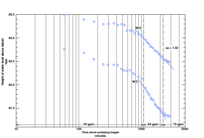
The well was pumped at 55 gpm for 1,098 minutes, and a cone of depression developed around the well and intersected the lake. The discharge rate was then increased to the maximum capacity of the well, 83 gpm, from 1,098 to 2,238 minutes. The well was then pumped at 70 gpm from 2,238 to 2,827 minutes, the end of the test.
Representative drawdown curves, illustrated by water-level measurements in wells W 2 and W 3, are shown in Figure 14. The changes in slope are readily observed to be coincident with changes in discharge. Equilibrium was approached near the end of the test. Although the nonartesian aquifer was being dewatered, use of the Theis modified nonequilibrium formula gives a reasonable estimate of transmissibility at well W 3, 120 feet from the pumped well. If the slope, Δ s, is 1.32 feet, and discharge, Q, is 83 gpm, then
T = (264) (83) / 1.32 = 17,000 gpd/ft.
Figure 14--Drawdown of water levels in observation well W 2 and W 3 during State Lake aquifer test. Datum is 1,200 feet above sea level.
Transmissibility computed from data at the end of the test, when the cone was approaching equilibrium, may be more reliable. Figure 15 shows the north and west profile of the cone of depression; the drawdown is plotted linearly against the distance of observation wells from the pumped well plotted logarithmically.
Figure 15--Profiles of cone of depression around pumped well being recharged by lake 200 feet away, during State Lake aquifer test. Datum is 1,200 feet above sea level.
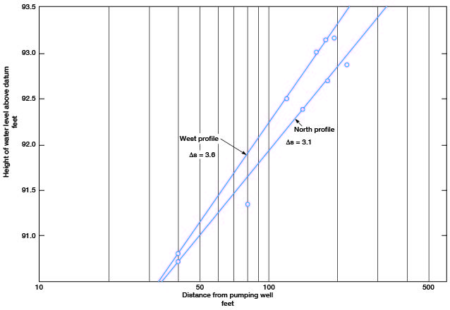
A modified form of the Thiem equation is
T = 528 Q / Δ s
If Q = 70 gpm and s - 3.1 feet, then
T = (528) (70) / 3.1
or T equals 12,000 and Pf equals 380.
Prev Page--Formations || Next Page--Hydrology
Kansas Geological Survey, Geology
Placed on web March 23, 2009; originally published January, 1962.
Comments to webadmin@kgs.ku.edu
The URL for this page is http://www.kgs.ku.edu/General/Geology/Ottawa/06_gw.html