---

Start
Contents
Introduction
Geography
Geology
Ground water
Geologic Formations
Hydrologic Properties
Summary
Well Records
Logs
References
Plates

Prev Page--Geologic Formations || Next Page--Summary

---

Hydrologic Properties of Water-bearing Materials

The quantity of water that a water-bearing formation will yield to wells depends upon the hydrologic properties of the material penetrated by the wells. The two hydrologic properties of greatest significance are the coefficients of transmissibility (T) and storage (S). These factors are used in making estimates of the quantity of water available in an aquifer and for predicting water-level decline resulting from continued pumping. Controlled aquifer tests in the field provide the data required to compute these coefficients.

The coefficient of transmissibility (T) may be defined as the number of gallons of water, at the prevailing temperature, that will move in 1 day through a vertical strip of the aquifer 1 foot wide, having a height equal to the full saturated thickness of the aquifer, under a hydraulic gradient of 100 per cent or 1 foot per foot.

The coefficient of storage (S) of an aquifer is the change in its stored volume of water per unit change in head per unit surface area of the aquifer. Under water-table conditions the coefficient of storage (S) is virtually the same as the specific yield of the aquifer.

The coefficient of permeability (P) of an aquifer is the discharge per unit of area per unit of hydraulic gradient. The field coefficient (Pf) may be measured in terms of the number of gallons of water a day, at the prevailing temperature, conducted laterally through each mile of aquifer under investigation (measured at right angles to the direction of flow) for each foot of thickness of the aquifer, and for each foot per mile of hydraulic gradient. The field coefficient of permeability multiplied by the thickness of the saturated water-bearing materials in feet, is equal to the coefficient of transmissibility.

Determinations of Transmissibility and Permeability

The coefficients of transmissibility and permeability of the alluvium and terrace deposits in the Republican River valley in Cloud County were determined by aquifer tests using three wells. Values for transmissibility were computed from the test data by the formulas developed by Theis, Thiem, and Cooper and Jacob.

Theis Recovery Method

The recovery method of determining the coefficient of transmissibility (Theis, 1935, p. 522) utilizes measurements of the water level in the pumped well during the recovery period. The Theis recovery formula is expressed as:

T = (264Q log₁₀ t/t') / s'

in which T is the coefficient of transmissibility, in gallons per day per foot, Q is the pumping rate, in gallons a minute, t is the time since pumping started, in minutes, t' is the time since pumping stopped, in minutes, and s' is the residual drawdown in the pumped well, in feet, at time t'.

The residual drawdown (s') is computed by subtracting the static water-level measurement from the measurement at time t' after pumping ceases.

The ratio of log₁₀ t/t' is determined graphically by plotting log₁₀ t/t' against corresponding value of s'. This procedure is simplified by plotting t/t' on the logarithmic coordinate and s' on the arithmetic coordinate of semilogarithmic paper. If log₁₀ t/t' is taken over 1 log cycle, it will become unity; s' will be the difference between drawdowns over 1 log cycle; and,the equation becomes T = (264Q / Δs). In practice, water levels at time t' may be plotted and the residual drawdown need not be computed. Inasmuch as the value of T is related directly to the slope of the line formed by plotting water level against t/t', the selection of the proper points on the plot to determine As is very important. Theoretically the relation of s' to t/t' should plot as a straight line that passes through the point where residual drawdown is 0 and where t/t' is 1. In unconsolidated deposits this is not always true, as the plotted line is a curve that does not. pass through the point of origin. The earliest points on the recovery curve may be erratic and may not fall in a straight line. This may be due in part to head losses in the well or to the surge of the column of water that falls back into the well after the pump is stopped. For this reason, the points where t/t' approaches 1 should be the most reliable and should be used in determining Δs, but the recovery data may not plot through the point where s' is 0 nor in a straight line in the later part of the test. It is then difficult to establish a line that determines Δs, and the latest data, where t/t' approaches 1, should not be used, but instead points earlier in the curve should be used. Where the data plot as an appreciable curve, almost any value can be obtained for As, and hence, the value of T can be considerably in error.

Thiem Method

The Thiem method of determining the coefficient of transmissibility of a water-bearing material consists of analyzing the decline in water level during the pumping period in several observation wells near the pumped well. After approximate equilibrium is established around a pumped well, approximately equal quantities of water move toward the pumped well per unit of time through a series of upright concentric cylindrical sections around the well. Because the areas of the large cylinders through which the water percolates are larger than the areas of the smaller cylinders, the velocity of the water percolating through the large cylinders is proportionately less than through the smaller cylinders and the hydraulic gradients are proportionately smaller. The Thiem formula is:

T = [527.7Q log₁₀(r₂/r₁)] / (s₁ - s₂)

in which T is the coefficient of transmissibility, in gallons per day per foot,
Q is the pumping rate, in gallons a minute,
r₁ and r₂ are distances of observation wells from pumped well, in any unit,
s₁ and s₂ are drawdowns of water level at distances r₁ and r₂ in feet.

When the values for drawdowns, s, are plotted on the arithmetic scale of semilogarithmic paper and the values for distances, r, are plotted on the logarithmic scale, the points fall on a straight line. For one log cycle, log₁₀(r₂/r₁) is equal to 1 and the Thiem formula becomes:

T = 527.7Q / Δs

where Δs is the drawdown over one log cycle.

The Thiem method of determining the coefficient of transmissibility is based on the theory that the aquifer is homogeneous throughout, but because aquifers are not actually perfectly homogeneous a probable error in the value of T is introduced. In some aquifer tests the aquifer is so heterogeneous that the drawdown rate is slowed in one or more of the observation wells and perhaps accelerated in others, thus giving a false slope to the line used in determining a value for Δs. Therefore it is advisable to utilize more than two observation wells to evaluate the results of an aquifer test by the Thiem method. In thin aquifers a correction should be applied to the observed drawdown. This correction factor is s² / 2m in which s is the observed drawdown and in is the saturated thickness of the aquifer. The observed drawdown is reduced by the amount of the correction.

Theis Nonequilibrium Method

The nonequilibrium formula introduced by Theis (1935) is:

or evaluating the integral

and s is the drawdown in an observation well, in feet,
r is the distance from pumped well to observation well, in feet,
Q is the discharge, in gallons per minute,
t is the time since pumping began, in days,
T is the coefficient of transmissibility, in gallons per day per foot,
S is the coefficient of storage.

The formula was developed on the basis of six theoretical assumptions: that the aquifer is infinite in extent, that it is homogeneous, that its transmissibility is constant at all places and in all directions, that it is confined between impermeable beds, that the coefficient of storage is constant, and that water is released instantaneously from storage with a decline in artesian head.

The exponential integral is often written symbolically as W(u), read as the "Well function of u," and its substitution in the equation results in the expression T = (114.6Q W(u)) / s. The presence of two unknowns and the nature of the exponential integral in the nonequilibrium formula make an exact analytical solution impossible. Solution can be obtained by the use of a graphical method of superposition devised by Theis.

To determine values of s, the extrapolated graph of water levels before pumping began is compared with the graph of the water levels after pumping began. Under static or near-static conditions, however, the drawdown s in the well may be plotted directly. These values of s are plotted on logarithmic paper along the vertical axis, the values of t being plotted along the horizontal axis where r is the distance from the pumped well and t is the time in days since pumping began. These points describe the "field curve." Generally u is plotted against W(u) to obtain a "type curve." In this report W(u) is plotted along the vertical axis against 1/u along the horizontal axis to yield a "type curve" of the same values except that it is reversed. This simplifies the plotting of the "field curve"' because many calculations may be omitted by plotting s against t instead of s against r²/t. Logarithmic paper of the same scale is used in plotting both the field curve and the type curve. If the basic assumptions are satisfied, the field curve will conform to a part of the type curve. A match of the two curves is obtained by superposing the field curve on the type curve, keeping the axes of the two parallel. With both curves in the matched position, a point on the type curve is selected and marked on the field curve. The coordinates of this common point, s, W(u), t, and 1/u, are then used to solve the nonequilibrium formula for T and S. For convenience a match point may be selected at the intersection of the major axes of the type curve, for example where W(u) = 1.0 and u = 0.1.

Cooper-Jacob Generalized Methods

The Theis (1935) nonequilibrium formula requires the use of a "type curve" on which the test-data curve is superimposed to determine the coefficients of transmissibility and storage. Cooper and Jacob (1946) devised three generalized graphical methods utilizing straight-line graphs. The three types of graphs are referred to as the generalized distance-drawdown graph, the generalized time-drawdown graph, and the generalized composite drawdown graph.

In the distance-drawdown graph, drawdown is plotted on the arithmetic scale and distance of observation wells in feet from the pumped well is plotted on the logarithmic scale. The formulas for coefficients of transmissibility and storage are:

T = 264Q / Δs and S = 0.3Tt / r₀²

In the time-drawdown graph, drawdown is plotted on the arithmetic scale and time in days is plotted on the logarithmic scale. The formulas for coefficients of transmissibility and storage are:

T = 264Q / Δs and S = 0.3Tt₀ / r²

In the composite drawdown graph, drawdown is plotted on the arithmetic scale and the value t/r² is plotted on the logarithmic scale. In this method the plots of all observation wells should fall on a straight line. The formulas for coefficients of transmissibility and storage are:

T = 264Q / Δs and S = 0.3T / (t / r²)₀

In the above formulas,
T is the coefficient of transmissibility, in gallons per day per foot,
S is the coefficient of storage,
Q is the rate of discharge of pumped well, in gallons per minute,
Δs is the drawdown over one log cycle,
t is the time since pumping started, in days,
r is the distance from pumped well, in feet,
t₀ is the value of t where drawdown = 0,
r₀ is the value of r where drawdown = 0,
t/r²)₀ is the value of t/r² where drawdown = 0.

Aquifer Tests

Three aquifer tests were made by pumping irrigation wells in the Republican River valley between Concordia and Clyde. The test in which well 5-2-25cb (W. T. Wright No. 1) was used was made in 1942 (Fishel, 1948). The tests in which well 5-2-25cc (W. T. Wright No. 2) and 6-1-4bbc on the Franklin Day farm were used were made in the fall of 1955. Wells 5-2-25cb and 5-2-25cc are in a wide bend of Republican River where the Wisconsinan terrace deposits have been developed extensively for irrigation. Geologically this area is very favorable for obtaining a good irrigation well. Well 6-1-4bbc is near the edge of the Republican Valley and is not favorably located for yielding a large ground-water supply.

W. T. Wright Well 5-2-25cb

An aquifer test using well 5-2-25cb was made in 1942. Observation wells were not available, and therefore the Theis recovery formula was applied to determine the coefficient of transmissibility of the aquifer. The well was pumped at a rate of 730 gpm from 8:28 a. m. to 2:40 p. m.; water-level measurements made during the pumping and recovery period are given in Table 6.

Table 6--Water-level measurements made during pumping and recovery of Wright well 5-2-25cb and values for t, t', and t/t'.

Time	Time since pumping started, minutes t	Time since pumping stopped, minutes t	t/t'	Depth to water, feet
8:20 a. m.	Static water level			18.43
8:28	Pumping started
8:40	12			30.32
9:10	42			30.55
9:40	72			30.59
10:45	137			30.62
11:40	192			30.55
1:00 p. m.	272			30.78
2:30	362			30.70
2:40	372 Pumping stopped
2:40:15.	372.25	0.25	1,489	24.13
2:41	373	1	373	20.51
2:42	374	2	137	19.64
2:42:30.	374.5	2.5	149.80	19.48
2:43	375	3	125	19.38
2:43:30	375.5	3.5	107.29	19.32
2:44	376	4	94	19.25
2:44:30	376.5	4.5	83.67	19.20
2:45	377	5	75.40	19.16
2:45:30	377.5	5.5	68.64	19.13
2:46	378	6	63	19.10
2:46:30	378.5	6.5	58.23	19.08
2:47	379	7	54.14	19.06
2:48	380	8	47.50	19.02
2:49	381	9	42.33	18.99
2:50	382	10	38.20	18.97
2:52	384	12	32.00	18.92
2:54	386	14	27.57	18.89
2:56	388	16	24.25	18.86
2:58	390	18	21.67	18.84
3:00	392	20	19.60	18.82
3:05	397	25	15.88	18.80
3:10	402	30	13.40	18.77
3:15	407	35	11.63	18.76
3:20	412	40	10.30	18.75
3:30	422	50	8.44	18.72
3:40	432	60	7.20	18.68
4:00	452	80	5.65	18.64
4:20	472	100	4.72	18.62
4:40	492	120	4.10	18.59
5:00	512	140	3.66	18.59
5:30	542	170	3.19	18.57

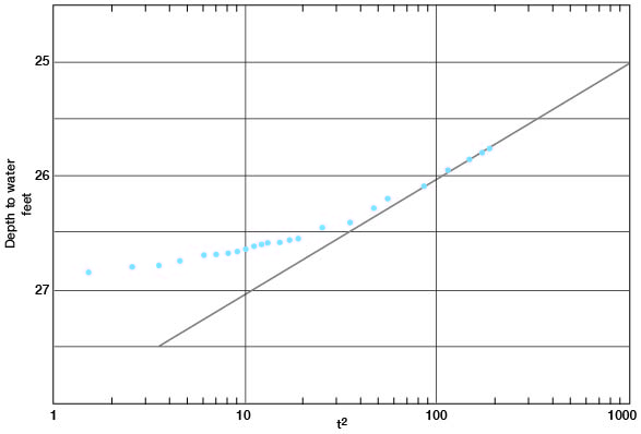
Figure 13--Depth to water in well 5-2-25cb plotted against t/t', time since pumping started divided by time since pumping stopped.

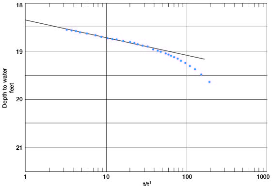
The ratio t/t' (time since pumping started, in minutes, divided by time since pumping stopped, in minutes) is plotted against the depth to water in Figure 13. From Figure 13 Δs, the change in water level over one log cycle, is 0.36. Hence,

T = [(264) (730)] / 0.36 = 540,000 gpd/ft.

The thickness, m, of the water-bearing material at the well is 47 feet, and from the relation P = T / m the coefficient of permeability (P) is 11,500. Drawdown was 12.27 feet at a pumping rate of 730 gpm, giving a specific capacity of 59.5 gpm per foot of drawdown for the well.

W. T. Wright Well 5-2-25cc

An aquifer test using well 5-2-25cc was made in the fall of 1955. Four observation wells, a, b, c, and d, were drilled 20.4, 51, 100, and 150 feet, respectively, from the pumped well. Well 5-2-25cc was pumped for 320 minutes at a rate of 1000 gpm. The water-level measurements made during the pumping and recovery periods and the values for t, t', and t/t' are given in Table 7.

Table 7--Water-level measurements made during pumping and recovery in Wright well 5-2-25cc and values for t, t' and t/t'.

Time	Time since pumping started, minutes t	Time since pumping stopped, minutes t	t/t'	Depth to water, feet
8:44 a.m.	Static water level			22.42
8:45	Pumping started
8:45:20	.33			31.20
8:46	1			31.72
8:46:30	1.5			31.90
8:47	2			31.94
8:47:30	2.5			31.97
8:48	3			32.01
8:49	4			32.03
8:50	5			32.10
8:51	6			32.17
8:52	7			32.22
8:53	8			32.26
8:54	9			32.30
8:55	10			32.31
8:58	13			32.31
9:00	15			32.31
9:05	20			32.32
9:10	25			32.34
9:15	30			32.38
9:20	35			32.39
9:30	45			32.47
9:40	55			32.50
9:45	60			32.57
10:00	75			32.62
10:10	85			32.66
10:30	105			32.71
10:45	120			32.78
11:04	139			32.86
11:20	155			32.90
11:35	170			32.90
11:50	185			32.91
12:05 p.m.	200			32.92
12:25	220			32.92
12:50	245			32.98
1:05	260			33.01
1:25	280			33.02
1:50	305			33.06
2:00	31~5			33.12
2:05	320 Pumping stopped
2:05:30	320.5	.5	641	23.75
2:05:45	320.75	.75	427.6	24.18
2:06	321	1 .	321	24.17
2:06:15	321.25	1.25	257	24.17
2:06:30 p. m.	321.5	1.5	214	24.11
2:06:45	321.75	1.75	183	24.10
2:07	322	2	161	24.09
2:07:30	322.5	2.5	129	24.08
2:08	323	3	107	24.07
2:08:30	323.5	3.5	92	24.05
2:09	324	4	81	24.04
2:10	325	5	65	24.01
2:11	326	6	54	23.99
2:12	327	7	46	23.97
2:13	328	8	41	23.95
2:14	329	9	36	23.92
2:15	330	10	33	23.90
2:17	332	12	27	23.87
2:19	334	14	24	23.85
2:22	337	17	20	23.82
2:25	340	20	17	23.78
2:28	343	23	15	23.75
2:31	346	26	13	23.73
2:34	349	29	12	23.69
2:39	354	34	10	23.65
2:44	359	39	9	23.61
2:49	364	44	8	23.59
3:00	375	55	7	23.51
3:05	380	60	6.3	23.49
3:10	385	65	5.9	23.47
3:15	390	70	5.5	23.44
3:25	400	80	5.0	23.41
3:35	410	90	4.5	23.36
3:45	420	100	4.20	23.33
3:55	430	110	3.90	23.32
4:10	445	125	3.56	23.26
4:25	460	140	3.28	23.21
4:40	475	155	3.06	23.16
4:55	490	170	2.88	23.12
5:10	505	185	2.73	23.09
5:25	520	200	2.60	23.08
5:30	525	205	2.55	23.06
7:10	625	305	2.04	22.95
7:40	655	335	1.95	22.89
8:10	685	365	1.87	22.87
8:40	715	395	1.81	22.84
9:25	760	440	1.72	22.81

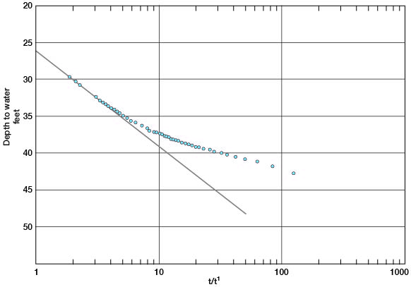
Figure 14--Depth to water in well 5-2-25cc plotted against t/t', time since pumping started divided by time since pumping stopped.

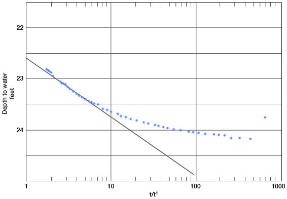
The ratio t/t' is plotted against depth to water on semilogarithmic paper in Figure 14. The points do not fall in a straight line, and the line drawn through the points does not go through the point of zero residual drawdown at the coordinate t/t'= 1. The points nearest t/t' = 1 give a value for T that is much lower than the value indicated by the observation wells; therefore, the line was arbitrarily drawn through the points where the values of t/t' were between 2 and 5. The line so drawn indicates a value of 1.15 for Δs. Applying the Theis recovery formula:

T = [(264) (1,000)] 1.15 / = 230,000 gpd/ft.

The thickness m is 47.6 feet, and from the relation p = T/m, P = 4,800 gpd/square foot. The drawdown at the end of the pumping period was 10.7 feet at 1,000 gpm, and thus the specific capacity was 93 gpm per foot of drawdown.

Depth-to-water measurements made in observation wells a, b, c, and d during the pumping period on well 5-2-25cc are given in Tables 8, 9, 10, and 11 respectively. Measurements made during the recovery period in observation well b are also given in Table 9.

Table 8--Water-level measurements in observation well a, 20.4 feet from pumped well 5-2-25cc.

Time	Time since pumping started, minutes t	t/r2	Depth to water, feet	Drawdown, feet
8:44 a.m.	Static water level		24.87
8:45	Pumping started
8:45:30	.5	1.2x10-3	25.79	.92
8:47	2	4.8x10-3	26.20	1.33
8:49	4	9.6x10-3	26.35	1.48
8:50	5	1.2x10-2	26.45	1.58
8:52	7	1.7x10-2	26.53	1.66
8:56	11	2.6x10-2	26.59	1.72
8:58	13	3.1x10-2	26.66	1.79
9:00	15	3.6x10-2	26.74	1.87
9:02	17	4.1x10-2	26.78	1.91
9:05	20	4.8x10-2	26.80	1.93
9:10	25	6.0x10-2	26.86	1.99
9:20	35	8.4x10-2	26.97	2.10
9:30	45	1.1x10-1	27.03	2.16
9:40	55	1.3x10-1	27.13	2.26
9:55	70	1.7x10-1	27.26	2.39
10:05	80	1.9x10-1	27.31	2.44
10:25	100	2.4x10-1	27.42	2.55
10:45	120	2.9x10-1	27.51	2.64
11:05	140	3.3x10-1	27.60	2.73
11:20	155	3.7x10-1	27.64	2.77
11:35	170	4.1x10-1	27.69	2.82
11:50	185	4.4x10-1	27.71	2.84
12:05 p.m.	200	4.8x10-1	27.77	2.90
12:25	220	5.3x10-1	27.80	2.93
12:45	240	5.8x10-1	27.86	2.99
1:05	260	6.2x10-1	27.91	3.04
1:25	280	6.7x10-1	28.00	3.13
1:50	305	7.3x10-1	28.02	3.15
2:05	Pumping stopped

Table 9--Water-level measurements in observation well b, 51 feet from pumped well 5-2-25cc.

Time	Time since pumping started, minutes t	Time since pumping stopped, minutes t'	t/r2	Depth to water, feet	Drawdown, feet
8:44 a. m.	Static water level			25.04
8:45	Pumping started
8:45:30	.5		1.9x10-4	25.44
8:46:30	1.5		5.7x10-4	25.66	.62
8:47:15	2.25		8.6x10-4	25.77	.73
8:48	3		1.1x10-3	26.88	.84
8:49	4		1.5x10-3	25.95	.91
8:50	5		1.9x10-3	26.02	.98
8:51	6		2.3x10-3	26.04	1.00
8:52	7		2.7x10-3	26.07	1.03
8:53	8		3.1x10-3	26.11	1.07
8:54	9		3.5x10-3	26.13	1.09
8:55	10		3.8x10-3	26,15	1.11
8:56	11		4.2x10-3	26.18	1.14
8:57	12		4.6x10-3	26.20	1.16
8:58	13		5.0x10-3	26.22	1.18
8:59	14		5.4x10-3	26.23	1.19
9:00	15		5.8x10-3	26.25	1.21
9:02	17		6.5x10-3	26.26	1.22
9:05	20		7.6x10-3	26.32	1.28
9:08	23		8.8x10-3	26.35	1.31
9:10	25		9.6x10-3	26.36	1.32
9:15	30		1.1x10-2	26.40	1.36
9:20	35		1.2x10-2	26.47	1.43
9:25	40		1.5x10-2	26.50	1.46
9:30	45		1.7x10-2	26.54	1.50
9:38	53		2.0x10-2	26.61	1.57
9:45	60		2.3x10-2	26.64	1.60
9:55	70		2.7x10-2	26.72	1.68
10:00	75		2.9x10-2	26.74	1.70
10:10	85		3.3x10-2	26.78	1.74
10:15	90		3.5x10-2	26.81	1.77
10:25	100		3.8x10-2	26.85	1.81
10:45	120		4.6x10-2	26.94	1.90
11:05	140		5.4x10-2	27.03	1.99
11:20	155		5.9x10-2	27.07	2.03
11:35	170		6.5x10-2	27.12	2.08
11:50	185		7.1x10-2	27.16	2.12
12:05 p.m.	200		7.7x10-2	27.20	2.16
12:25	220		8.4x10-2	27.24	2.20
12:45 p.m.	240		9.2x10-2	27.29	2.25
1:05	260		1.0x10-1	27.33	2.29
1:25	280		1.1x10-1	27.38	2.34
1:50	305		1.2x10-1	27.43	2.39
2:05	Pumping stopped
2:05:30	305.5	.5		26.86
2:07:30	307.5	2.5		26.81
2:08:30	308.5	3.5		26.78
2:09:30	309.5	4.5		26.75
2:11	311	6		26.70
2:12	312	7		26.69
2:13	313	8		26.68
2:14	314	9		26.66
2:15	315	10		26.63
2:16	316	11		26.61
2:17	317	12		26.60
2:18	318	13		26.59
2:20	320	15		26.58
2:22	322	17		26.56
2:24	324	19		26.55
2:30	330	25		26.46
2:40	340	35		26.36
2:52	352	47		26.28
3:00	360	55		26.22
3:30	390	85		26.09
4:00	420	115		25.96
4:30	450	145		25.87
5:00	480	175		25.80
5:13	493	188		25.77

Table 10--Water-level measurements in observation well c, 100 feet from pumped well 5,2-25cc.

Time	Time since pumping started, minutes t	t/r2	Depth to water, feet	Drawdown, feet
8:44 a.m.	Static water level		22.45
8:45	Pumping started
8:45:30	.5	5.0x10-5	22.55	.10
8:46:30	1.5
8:47:30	2.5	2.5x10-4	22.73	.28
8:48:30	3.5	3.5x10-4	22.85	.40
8:49:30	4.5	4.5x10-4	22.88	.43
8:50:30	5.5	5. 5x10-4	22.97	.52
8:52	7	7.0x10-4	23.02	.57
8:53	8	8.0x10-4	23.06	.61
8:54	9	9.0x10-4	23.09	.64
8:56	11	1.1x10-3	23.13	.68
8:58	13	1.3x10-3	23.17	.72
9:00	15	1.5x10-3	23.20	.75
9:03	18	1.8x10-3	23.24	.79
9:05	20	2.0x10-3	23.27	.82
9:10	25	2.5x10-3	23.31	.86
9:15	30	3.0x10-3	23.35	.90
9:25	40	4.0x10-3	23.42	.97
9:35	50	5.0x10-3	23.48	1.03
9:45	60	6.0x10-3	23.50	1.05
9:55	70	7.0x10-3	23.59	1.14
10:05	80	8.0x10-3	23.63	1.18
10:15	90	9.0x10-3	23.63	1.18
10:25	100	1. Ox10-2	23.68	1.23
10:45	120	1.2x10-2	23.77	1.32
11:05	140	1.4x10-2	23.82	1.37
11:20	155	1.5x10-2	23.85	1.40
11:35	170	1.7x10-2	23.90	1.45
11:50	185	1.8x10-2	23.93	1.48
12:05 p. m.	200	2.0x10-2	23.97	1.52
12:25	220	2.2x10-2	24.02	1.57
12:45	240	2.4x10-2	24.05	1.60
1:05	260	2.6x10-2	24.09	1.64
1:25	280	2.8x10-2	24.11	1.66
1:50	305	3.1x10-2	24.12	1.67

Table 11--Water-level measurements in observation well d, 150 feet from pumped well 5-2-25cc.

Time	Time since pumping started, minutes t	t/r2	Depth to water, feet	Drawdown, feet
8:44 a. m.	Static water level		23.95
8:45	Pumping started
8:48	3	1.3x10-4	24.13	.18
8:50	5	2.2x10-4	24.29	.34
8:52	7	3.1x10-4	24.36	.41
8:54	9	4.0x10-4	24.43	.48
8:56	11	4.9x10-4	24.50	.55
8:58	13	5.8x10-4	24.50	.55
9:00	15	6.6x10-4	24.57	.62
9:03	18	8.0x10-4	24.59	.64
9:05	20	8.8x10-4	24.57	.62
9:10	25	1.1x10-3	24.60	.65
9:15	30	1.3x10-3	24.60	.65
9:25	40	1.7x10-3	24.73	.78
9:35	50	2.2x10-3	24.80	.85
9:45	60	2.7x10-3	24.81	.86
9:55	70	3.1x10-3	24.85	.90
10:05	80	3.5x10-3	24.88	.93
10:15	90	4.0x10-3	24.90	.95
10:25	100	4.4x10-3	24.95	1.00
10:45	120	5.3x10-3	24.98	1.03
11:05	140	6.2x10-3	25.04	1.09
11:20	155	6.9x10-3	25.06	1.11
11:35	170	7.5x10-3	25.09	1.14
11:50	185	8.2x10-3	25.13	1.18
12:05 p. m.	200	8.8x10-3	25.15	1.20
12:25	220	9.8x10-3	25.18	1.23
12:45	240	1.1x10-2	25.23	1.28
1:05	260	1.2x10-2	25.25	1.30
1:25	280	1.3x10-2	25.28	1.33
1:50	305	1.4x10-2	25.32	1.37
2:05	Pumping stopped

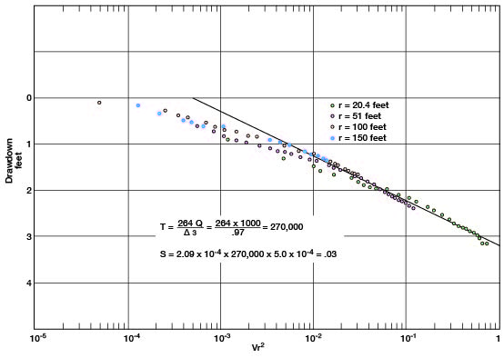
Drawdown measurements in observation wells a, b, c, and d are plotted against t/r² in the composite straight-line graph shown in Figure 15. A line drawn using the later data from each of the observation wells gives a value of 0.97 for Δs. Applying the Cooper-Jacob composite generalized formula:

T= [(264) (1,000)] / 0.97 = 270,000 gpd/ft.

and

S = (2.09 X 10^-4) (270,000) (5.0 X 10^-4) = 0.03

Figure 15--Drawdown in observation wells a, b, c, and d, plotted against t/r², in aquifer test using well 5-2-25cc.

In Figure 16 the depth-to-water measurements made during the recovery period in observation well b are plotted against the time since pumping stopped. A line through the late points in the recovery period gives a value of 1.0 for Δs; applying the Cooper-Jacob generalized time-drawdown formula:

T = [(264) (1,000)] 1.0 / = 260,000 gpd/ft.

Figure 16--Depth to water in observation well b plotted against time since pumping started (t) or stopped (t') in well 5-2-25cc.

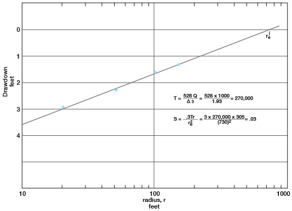
The corrected drawdowns in observation wells a, b, c, and d at 305 minutes after pumping began are plotted in Figure 17 against distance of the observation wells from the pumped well 5-2-25cc. A line through these points gives a value of 2.12 for As; applying the Thiem formula:

T = [(528) (1,000)] / 2.12 = 270,000

and

S = [(0.3) (270,000) (305)] / (730)² = 0.03

Figure 17--Drawdowns in observation wells a, b, c, and d at 305 minutes after pumping started plotted against distance (r) of observation wells from pumped well 5-2-25cc.

Summary of Wright Aquifer Tests

The value of the coefficient of transmissibility (T) obtained from the test on well 5-2-25cb was 540,000 gpd per foot. From the test using well 5-2-25cc, values for T were obtained by the Theis recovery method, the Thiem method, and the Cooper-Jacob generalized composite method. These values ranged from 230,000 gpd per foot in the pumped well, as computed by the Theis recovery method, to 270,000 gpd per foot by the Thiem method. The value for T obtained by the Theis recovery method is probably in error because the points in Figure 14 do not fall in a straight line. The value for T obtained from well 5-2-25cb seems to be too high, as the geologic conditions at wells 5-2-25cb and 5-2-25cc are very similar and would not indicate as great a difference. The values of T obtained by the Cooper-Jacob generalized composite method, the Thiem method, and the modified nonequilibrium method on well 5-2-25cc are all in fair agreement and probably are near the true value for T in this area. The values obtained for the coefficient of storage (S) indicate water-table conditions in the vicinity of the well. The values of S probably are much less than the true value of the storage coefficient. In a longer test the value of S would continue to increase until a nearly true value could be obtained.

Franklin Day Well 6-1-4bbc

An aquifer test was made by pumping well 6-1-4bbc in the fall of 1955. The well was pumped for a period of 245 minutes at a rate of 540 gpm. Three observation wells, a, b, and c, were drilled at distances of 48 feet, 100 feet, and 147 feet, respectively, from the pumped well, and drawdown measurements were made during the period of pumping. The water-level measurements made in well 6-1-4bbc during the drawdown and recovery periods, and values for t, t', and t/'t, are given in Table 12.

Table 12--Water-level measurements made during pumping and recovery in Day well 6-1-4bbc and values for t, t, and t/t'.

Time	Time since pumping started, minutes t	Time since pumping stopped, minutes t'	t/t'	Depth to water, feet
12:25 p.m.	Static water level			26.05
12:30	Pumping started
12:30:20	.3			37.80
12:30:4	.75			40.80
12:31	1			42.55
12:32	2			45.00
12:32:30	2.5			46.50
12:33	3			47.60
12:34	4			48.30
12:35	5			51.30
12:36	6			52.40
12:37	7			53.48
12:38	8			54.80
12:39	9			55.52
12:40	10			56.09
12:45	15			58.44
12:50	20			60.51
12:55	25			62.75
1:00	30			64.45
1:10	40			65.14
1:21	51			66.05
1:30	60			66.06
4:35	245	Pumping stopped
4:37	247	2	123	42.71
4:38	248	3	83	41.72
4:39	249	4	62	41.18
4:40	250	5	50	40.81
4:41	251	6	42	40.50
4:42	252	7	36	40.22
4:43	253	8	32	39.98
4:44	254	9	28	39.74
4:45	255	10	26	39.55
4:46	256	11	23	39.41
4:47	257	12	21	39.26
4:48	258	13	20	39.11
4:49	259	14	18.5	38.97
4:50	260	15	17.3	38.83
4:51	261	16	16.3	38.70
4:52	262	17	15.4	38.56
4:53	263	18	14.6	38.44
4:54 p.m.	264	19	13.9	38.33
4:55	265	20	13.2	38.22
4:56	266	21	12.7	38.10
4:57	267	22	12.1	37.99
4:58	268	23	11.7	37.86
4:59	269	24	11.2	37.77
5:00	270	25	10.8	37.66
5:01	271	26	10.4	37.55
5:02	272	27	10.1	37.45
5:03	273	28	9.7	37.34
5:04	274	29	9.4	37.23
5:05	275	30	9.18	37.13
5:07	277	32	8.15	36.93
5:10	280	35	8.00	36.67
5:15	285	40	7.12	36.25
5:20	290	45	6.45	35.86
5:25	295	50	5.90	35.53
5:30	300	55	5.46	35.22
5:35	305	60	5.08	34.93
5:40	310	65	4.77	34.66
5:45	315	70	4.50	34.40
5:50	320	75	4.27	34.14
5:56	326	81	4.02	33.88
6:00	330	85	3.88	33.68
6:06	336	91	3.70	33.45
6:15	345	100	3.45	33.11
6:25	355	110	3.23	32.80
6:35	365	120	3.04	32.50
7:53	443	198	2.24	30.83
8:25	475	230	2.07	30.35
9:30	540	295	1.83	29.65
8:50 a.m.	1,220	975	1.25	27.26

The ratio t/t' is plotted against depth to water (s') on semilogarithmic paper in Figure 18. The later points, as plotted, seem to fall on a straight line that approaches the zero-drawdown point where t/t' = 1. This line gives a value for Δs of 13.0. Applying the Theis recovery formula (T = 264Q / Δs'), T = 11,000 gpd/ft.; but the data from the observation wells indicate that this value is too low, probably because of entrapped air, which could be heard escaping for a considerable period after pumping stopped. Presumably the water level did not recover as rapidly as it would have if air had not been entrapped, and the plotted line based on observed water levels therefore is displaced somewhat from its expectable position. Hence, T as calculated may be in error. An arbitrary line can be drawn through the values of t/t' from about 3.5 to 6, which will give 13,000, a value for T that more nearly equals the value obtained from the observation-well data. The thickness of saturated material (m) at the well is 43 feet; hence, from the relation P = T/m the permeability is computed to be 300 gpd per square foot. The specific capacity is 13.5 gpm per foot of drawdown.

Figure 18--Depth to water in well 6-1-4bbc plotted against t/t', time since pumping started divided by time since pumping stopped.

Drawdown measurements made in observation well a during the pumping period are given in Table 13. Observation well a was 48 feet from pumped well 6-1-4bbc. The data in Table 13 are plotted on logarithmic paper in Figure 19, the time since pumping started (t) being plotted along the horizontal axis and the drawdown (s) along the vertical axis. The match point on the type curves gives s = 8.3 and t = 17.8 minutes. Using the Theis nonequilibrium formulas where T = (208.5Q) / s and S = [3.71 X 10^-5 (Tt)] / r², T = 13,500 gpd/foot and S = 0.003. The value for S = 0.003 indicates a semiartesian or a slow-draining condition.

Figure 19--Drawdown of water level in observation well a plotted against time since pumping started (t) in well 6-1-4bbc.

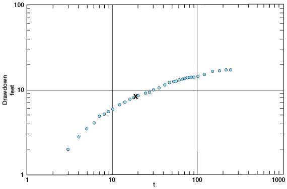
Table 13--Water-level measurements in observation well a, 48 feet from pumped well 6-1-4bbc.

Time	Time since pumping started, minutes t	Depth to water, feet
12:26 p.m.	Static water level	26.66
12:30	Pumping started
12:31	1	27.05
12:32	2	27.52
12:33	3	28.69
12:34	4	29.49
12:35	5	30.22
12:36	6	30.82
12:37	7	31.66
12:38	8	31.95
12:39	9	32.34
12:40	10	32.70
12:42	12	33.31
12:44	14	33.89
12:46	16	34.44
12:48	18	34.86
12:50	20	35.27
12:54	24	36.00
12:57	27	36.43
1:00	30	36.86
1:05	35	37.49
1:11	41	38.11
1:16	46	38.69
1:21	51	39.13
1:25	55	39.40
1:30	60	39.70
1:35	65	39.96
1:40	70	40.19
1:45	75	40.44
1:50	80	40.72
1:55	85	40.90
2:00	90	41.10
2:11	101	41.38
2:20	110	41.63
2:30	120	41.84
2:40	130	42.05
2:52	142	42.25
3:00	150	42.42
3:15	165	42.61
3:30	ISO	42.79
3:45	195	42.94
4:00	210	43.04
4:15	225	43.15
4:30	240	43.20
4:35	Pumping stopped

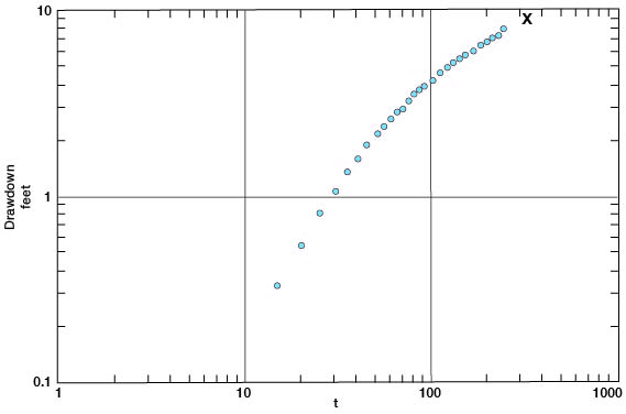
Drawdown measurements made in observation well b during the pumping period in well 6-1-4bbc are given in Table 14. Observation well b was 100 feet from the pumped well. The drawdown data are plotted on logarithmic paper in Figure 20, the time in minutes along the horizontal axis and the drawdown along the vertical axis. The match point on the type curve gives s = 9.0 and t = 43 minutes. Using the Theis nonequilibrium formulas applied in the preceding paragraph, T = 12,500 gpd/ft. and S = 0.001.

Figure 20--Drawdown of water level in observation well b plotted against time since pumping started (t) in well 6-1-4bbc.

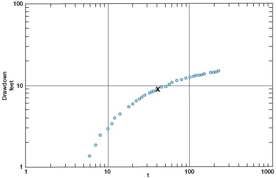
Table 14--Water-level measurements in observation well b, 100 feet from pumped well 6-1-4bbc.

Time	Time since pumping started, minutes t	Depth to water, feet
12:26 p.m.	Static water level	25.88
12:30	Pumping started
12:31	1	25.89
12:32	2	25.92
12:33	3	26.20
12:34	4	26.49
12:35	5	26.86
12:36	6	27.23
12:37	7	27.76
12:38	8	28.23
12:40	10	28.84
12:41	11	29.28
12:42	12	29.93
12:44	14	30.36
12:48	18	31.41
12:50	20	31.82
12:52	22	32.39
12:54	24	32.71
12:56	26	33.18
12:58	28	33.47
1:02	32	33.98
1:04	34	34.22
1:06	36	34.53
1:10	40	34.93
1:15	45	35.45
1:21	51	35.75
1:26	56	36.45
1:31	61	36.78
1:36	66	37.10
1:41	71	37.35
1:46	76	37.62
1:52	82	37.87
1:57	87	38.08
2:01	91	38.24
2:11	101	38.58
2:21	111	38.85
2:30	120	39.11
2:40	130	39.40
2:50	140	39.60
3:00	150	39.82
3:15	165	40.05
3:30	180	40.27
3:45	195	40.45
4:00	210	40.60
4:15	225	40.74
4:30	240	40.82
4:35	245 Pumping stopped

Drawdown data for observation well c obtained during the pumping period of well 6-1-4bbc are given in Table 15 and plotted on logarithmic paper, the time (t) being plotted along the horizontal axis and the drawdown (s) along the vertical axis (Fig. 21). The match point on the type curve gives s = 8.6 and t = 28 minutes. Using the Theis nonequilibrium formulas applied for wells a and b, T = 13,000 gpd/ft. and S = 0.006.

Table 15--Water-level measurements in observation well c, 147 feet from pumped well 6-1-4bbc.

Time	Time since pumping started, minutes t	Depth to water, feet
12:23 p. m.	Static water level	26.82
12:30	Pumping started
12:31	1	26.82
12:40	10	26.89
12:45	15	27.16
12:50	20	27.38
12:55	25	27.60
1:00	30	27.86
1:05	35	28.13
1:10	40	28.40
1:15	45	28.90
1:21	51	28.97
1:25	55	29.18
1:30	60	29.40
1:35	65	29.64
1:40	70	29.70
1:45	75	30.08
1:50	80	30.33
1:55	85	30.52
2:00	90	30.69
2:10	100	31.06
2:20	110	31.42
2:30	120	31.69
2:40	130	32.00
2:50	140	32.32
3:00	150	32.58
3:15	165	32.93
3:30	180	33.29
3:45	195	33.63
4:00	210	33.81)
4:15	225	34.16
4:30	240	34.85
4:35	Pumping stopped

Figure 21--Drawdown of water level in observation well c plotted against time since pumping started (t) in well 6-1-4bbc.

Summary of Day Aquifer Test

The results from the Day aquifer test using three observation wells are in fair agreement, and the values for T and S are accurate within practical limits. Calculations based on the data obtained during the test indicate that the pumping rate during the test was excessive and pumping could not continue very long at this rate. The well probably could be pumped at a rate of 400 gpm for a period of about 10 days before the yield would decline appreciably. Inasmuch as the well is used for short periods of continuous pumping and is then allowed to recover for several days, a discharge rate of about 400 gpm, though it could not be safely exceeded, probably could be maintained.

---

Prev Page--Geologic Formations || Next Page--Summary

Kansas Geological Survey, Geology
Placed on web June 29, 2009; originally published May 1959.
Comments to webadmin@kgs.ku.edu
The URL for this page is http://www.kgs.ku.edu/General/Geology/Cloud/07_prop.html