![]()
Prev Page--Ground water recharge, discharge, utilization || Next Page--Rock units
Ground Water
Chemical Character of Water
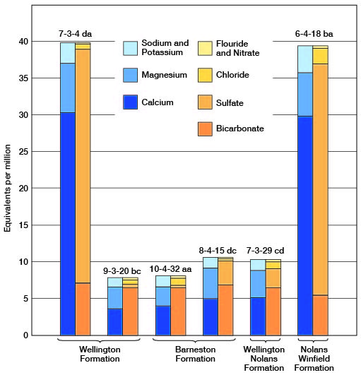
The chemical character of the ground water in Clay County is indicated by the analyses of 33 samples (2 composite) of water from 35 wells and test holes distributed as uniformly as practicable within the area and among the principal water-bearing formations (Table 3). A graphic representation of the chemical analyses of water from representative wells in the county is shown in Figures 8 and 9.
The depth given in Table 3 for the samples of water from test holes is the depth from which the sample was pumped. For all other samples of water the depth indicated is the total depth of the well. The samples of water were analyzed by Howard A. Stoltenberg, chemist, in the Water and Sewage Laboratory of the Kansas State Board of Health.
Table 3--Analyses of water from typical wells, springs, and test holes in Clay County. Analyzed by H. A. Stoltenberg. Dissolved constituents given in parts per million. (One part per million is equivalent to one pound of substance per million pounds of water or 8.33 pounds per minion gallons of water.)
| Location | Depth, feet |
Geologic source | Date of collection |
Temp. (°F) |
Dissolved solids |
Silica (SiO2) |
Iron (Fe) |
Calcium (Ca) |
Magnesium (Mg) |
Sodium and Potassium (Na + K) |
Bicarbonate (HCO3) |
Sulfate (SO4) |
Chloride (Cl) |
Fluoride (F) |
Nitrate (NO3) |
Hardness as CaCO3 | ||
|---|---|---|---|---|---|---|---|---|---|---|---|---|---|---|---|---|---|---|
| Total | Carbonate | Non- carbonate |
||||||||||||||||
| 6-1-2bac1 | 65 | Terrace deposits | 7-20-1945 | 58 | 345 | 24 | 0.61 | 70 | 12 | 37 | 290 | 40 | 16 | 0.3 | 1.5 | 224 | 224 | 0 |
| 6-1-2cc | 56-61 | Alluvium | 6-17-1954 | 58 | 373 | 28 | 3.8 | 88 | 13 | 29 | 345 | 26 | 18 | 0.3 | 0.9 | 273 | 273 | 0 |
| 6-1-15da | 56-61 | Terrace deposits | 6-18-1954 | 57 | 367 | 28 | 0.88 | 75 | 11 | 42 | 303 | 33 | 28 | 0.3 | 0.8 | 232 | 232 | 0 |
| 6-2-3ad | 59 | Dakota Formation | 10-26-1954 | 56 | 571 | 14 | 18 | 100 | 17 | 78 | 261 | 54 | 121 | 0.3 | 58 | 320 | 214 | 106 |
| 6-2-32ccc | 60-65 | Alluvium | 6-23-1954 | 56 | 1,320 | 18 | 4.1 | 315 | 32 | 57 | 300 | 721 | 30 | 0.6 | 2.3 | 918 | 246 | 672 |
| 6-2-33cd | 56-61 | Terrace deposits | 6-24-1954 | 525 | 23 | 1.2 | 122 | 19 | 30 | 317 | 160 | 13 | 0.4 | 1.7 | 382 | 260 | 122 | |
| 6-4-18ba | 77 | Nolans and Winfield Limestones | 10-26-1954 | 56 | 2,530 | 10 | 11 | 601 | 71 | 83 | 349 | 1,510 | 77 | 0.8 | 1.5 | 1,790 | 286 | 1,500 |
| 6-4-33ad | 103 | Barneston Limestone | 10-26-1954 | 55 | 431 | 13 | 0.50 | 76 | 47 | 20 | 459 | 13 | 10 | 0.3 | 26 | 382 | 376 | 6 |
| 7-1-6bb | 74-76 | Dakota Formation | 7-8-1954 | 502 | 9.5 | 89 | 27 | 53 | 337 | 134 | 20 | 0.4 | 3.2 | 333 | 276 | 57 | ||
| 7-1-15bcb | 65 | Dakota Formation | 6-9-1954 | 57 | 853 | 8.2 | 4.9 | 145 | 23 | 106 | 262 | 54 | 171 | 0.2 | 217 | 456 | 215 | 241 |
| 7-1-19bc | 50 | Dakota Formation | 3-4-1954 | 54 | 174 | 7.4 | 5.4 | 20 | 4.6 | 35 | 68 | 31 | 37 | 0.2 | 6.2 | 69 | 56 | 13 |
| 7-2-4ddc | 57 | Terrace deposits | 11-24-1953 | 514 | 0.18 | 122 | 24 | 28 | 354 | 140 | 16 | 0.3 | 6.6 | 403 | 290 | 113 | ||
| 7-3-4da | Spring | Wellington Formation | 3-1-1954 | 57 | 2,540 | 17 | 0.42 | 608 | 83 | 60 | 432 | 1,530 | 25 | 0.8 | 1.5 | 1,860 | 354 | 1,500 |
| 7-3-29cd | 77 | Wellington Formation and Nolans Ls. | 10-26-1954 | 55 | 574 | 18 | 0.10 | 107 | 44 | 34 | 407 | 121 | 34 | 0.4 | 16 | 448 | 334 | 114 |
| *7-4-20ad *7-4-21bc |
190 | Barneston Limestone | 3-2-1954 | 835 | 15 | 0.23 | 143 | 67 | 39 | 368 | 311 | 49 | 0.6 | 26 | 632 | 302 | 330 | |
| 7-4-32cc | 195 | Barneston Limestone | 10-26-1954 | 56 | 568 | 10 | 15 | 107 | 50 | 26 | 429 | 143 | 18 | 0.8 | 1.7 | 472 | 352 | 120 |
| 8-1-13ca | 40 | Terrace deposits | 10-13-1955 | 889 | 32 | 0.77 | 160 | 35 | 44 | 261 | 246 | 79 | 0.3 | 71 | 543 | 214 | 329 | |
| 8-2-30dd | Dakota Formation | 6-9-1954 | 56 | 1,140 | 9.4 | 3.2 | 151 | 88 | 97 | 295 | 146 | 244 | 0.6 | 261 | 738 | 242 | 496 | |
| 8-3-8db | 58 | Terrace deposits | 1-31-1948 | 655 | 30 | 3.5 | 144 | 24 | 29 | 445 | 125 | 15 | 0.4 | 5.3 | 458 | 365 | 93 | |
| 8-3-35da2 | 16-21 | Alluvium | 6-29-1954 | 58 | 330 | 12 | 75 | 20 | 18 | 294 | 47 | 11 | 0.4 | 1.1 | 269 | 241 | 28 | |
| 8-4-15dc | 118 | Barneston Limestone | 10-26-1954 | 56 | 580 | 13 | 9.0 | 102 | 51 | 32 | 427 | 157 | 13 | 0.6 | 1.3 | 464 | 350 | 114 |
| 9-2-30bb | Spring | Dakota Formation | 10-27-1954 | 57 | 58 | 11 | 0.23 | 7.4 | 1.8 | 7.6 | 29 | 4.9 | 7.0 | 0.2 | 3.6 | 26 | 24 | 2 |
| 9-3-1cc | 93 | Barneston Limestone | 10-26-1954 | 55 | 546 | 18 | 2.0 | 100 | 37 | 46 | 454 | 93 | 16 | 0.4 | 12 | 402 | 372 | 30 |
| 9-3-20bc | 78 | Wellington Formation; | 6-9-1954 | 56 | 401 | 11 | 1.9 | 75 | 36 | 26 | 404 | 18 | 20 | 0.2 | 16 | 335 | 331 | 4 |
| 9-3-23cc | 99 | Barneston Limestone | 10-26-1954 | 56 | 407 | 20 | 1.5 | 84 | 38 | 16 | 456 | 9.1 | 10 | 0.2 | 4.4 | 366 | 366 | 0 |
| 9-4-21aa | 144 | Barneston Limestone | 10-26-1954 | 55 | 371 | 16 | 0.26 | 76 | 23 | 32 | 383 | 14 | 14 | 0.2 | 6.6 | 284 | 284 | 0 |
| 9-4-32adc | 31-36 | Terrace deposits | 7-1-1954 | 57 | 278 | 22 | 67 | 9.5 | 19 | 254 | 28 | 6.0 | 0.4 | 1.3 | 206 | 206 | 0 | |
| 10-1-17dc | 100 | Dakota Formation | 5-16-1944 | 119 | 11 | 1.2 | 16 | 3.8 | 12 | 70 | 13 | 5.0 | 0.1 | 2.2 | 56 | 56 | 0 | |
| 10-2-17cd | 55 | Terrace deposits | 6-9-1954 | 56 | 3,600 | 22 | 29 | 198 | 549 | 292 | 371 | 2,170 | 178 | 0.9 | 1.9 | 2,180 | 304 | 1,880 |
| 10-2-23bb | 65 | Nolans Limestone | 6-9-1954 | 57 | 476 | 9.4 | 1.5 | 73 | 31 | 64 | 387 | 46 | 54 | 0.2 | 8.4 | 310 | 310 | 0 |
| 10-3-13ba | 107 | Barneston Limestone | 10-26-1954 | 55 | 668 | 14 | 1.5 | 98 | 40 | 77 | 366 | 90 | 76 | 0.3 | 93 | 409 | 300 | 109 |
| *10-4-5db1 *10-4-5db2 |
57 | Terrace deposits | 8-11-1954 | 605 | 25 | .04 | 109 | 28 | 40 | 371 | 56 | 43 | 0.2 | 62 | 387 | 304 | 83 | |
| 10-4-32aa | 134 | Barneston Limestone | 10-26-1954 | 56 | 427 | 16 | 1.7 | 84 | 30 | 34 | 398 | 16 | 36 | 0.2 | 15 | 333 | 326 | 7 |
| *Composite sample from two wells. | ||||||||||||||||||
Figure 8--Graphic representation of chemical analyses of water from principal water-bearing formations in representative wells in Clay County.
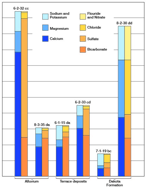
Figure 9--Graphic representation of chemical analyses of water from minor water-bearing formations in representative wells in Clay County.
Chemical Constituents in Relation to Use
The following discussion of the chemical constituents of ground water has been adapted from publications of the State Geological Survey of Kansas. The analyses of samples of water collected in Clay County are given in Table 3.
Dissolved solids--The residue left after a natural water has evaporated consists of rock materials, but may include some organic material and water of crystallization. Waters containing less than 500 parts per million of dissolved solids generally are satisfactory for domestic use, except for difficulties resulting from hardness and, in some cases, excessive iron content or corrosiveness. Waters having more than 1,000 ppm are as a rule not satisfactory, for they are likely to contain enough of certain constituents to produce a noticeable taste or to make the water unsuitable in some other respect.
The concentration of dissolved solids was less than 500 ppm in 14 of the 33 samples of water collected in Clay County, ranged from 500 to 1,000 ppm in 14 samples, and was more than 1,000 ppm in 5 samples. The water sample having the lowest concentration of dissolved solids (58 ppm) was from a spring (9-2-30bb) in the Dakota Formation. The water sample having the highest concentration of dissolved solids (3,600 ppm) was from well 10-2-17cd1 in the Wisconsinan terrace deposits. This sample had a very high concentration of calcium and sulfate ions.
Hardness--The hardness of water, which is the property of water that generally receives the most attention, is most commonly recognized by its effects when soap is used with water. Hard water is objectionable because it forms with soap a sticky, insoluble curd difficult to remove from containers and fabrics, and because it requires much soap to form a lather. Hard water forms scale in boilers and pipes, which reduces efficiency of heat transfer and may even result in boiler failure. Calcium and magnesium cause most of the hardness of ordinary water, and hence also the greater part of the scale in steam boilers and in other vessels in which water is heated or evaporated.
In addition to total hardness the table of analyses shows carbonate hardness and noncarbonate hardness. The carbonate hardness is that due to the presence of calcium and magnesium bicarbonates. It may be almost completely removed by boiling. This type of hardness has been called temporary hardness. The noncarbonate hardness is due to the presence of the sulfates or chlorides of calcium and magnesium and cannot be removed by boiling, and for this reason has sometimes been called permanent hardness. With reference to use with soap there is no difference between the carbonate and noncarbonate hardness.
Water having a hardness of less than 50 ppm is generally considered soft, and under ordinary circumstances treatment for removal of hardness is not necessary. Hardness between 50 and 150 ppm does not seriously interfere with the use of water for most purposes, but it does increase somewhat the consumption of soap, and its removal by a softening process is profitable for laundries and other industries using large quantities of soap. Hardness of more than 150 ppm can be noticed by most users, and if the hardness is 200 ppm or more the water is commonly softened. Where municipal water supplies are softened, an attempt is generally made to reduce the hardness to about 80 to 100 ppm. Further softening of a public supply is deemed not worth the additional cost.
Of the 33 samples of water collected in Clay County only 3 samples had a hardness of less than 150 ppm, and these 3 samples were from the Dakota Formation. Six samples had a hardness of 150 to 300 ppm, and 24 samples had a hardness of more than 300 ppm. All but one of the samples collected from wells in Permian rocks had a hardness of more than 300 ppm.
Iron--If the water contains much more than 0.3 ppm of iron, the excess may separate out and settle as a reddish sediment when exposed to air. Iron may be present in sufficient quantity to give a disagreeable taste or to stain cooking utensils; it may be removed by aeration and filtration, but some water requires additional treatment to remove the iron.
Water samples from the test holes in Clay County were pumped by the air-lift method, and the resulting aeration resulted in precipitation of much of the iron. These samples were not analyzed for iron. Only 6 of the 30 samples of water from Clay County that were analyzed for iron contained less than 0.3 ppm.
Fluoride--The fluoride content of water used by children should be known, because fluoride in water has been shown to be associated with the dental defect known as mottled enamel. Mottled enamel may appear on the teeth of children who, during the formation of the permanent teeth, drink water containing excessive amounts of fluoride. According to standards promulgated by the U. S. Public Health Service (1946), water containing more than 1.5 ppm of fluoride should not be used by children. If water contains as much as 4 ppm of fluoride, 90 percent of the children habitually drinking it are likely to have mottled enamel. Concentrations of fluoride of about 1 to 1.5 ppm have been shown to be beneficial in reducing tooth decay, and fluoride is now being added to some municipal supplies to bring the concentration up to about 1 to 1.5 ppm. The water samples collected in Clay County had a fluoride content of less than 1 ppm.
Chloride--Chloride is widely distributed in nature; it is an abundant constituent of sea water and oil-field brines and is dissolved from most rock materials. Chloride has little effect on the suitability of water for ordinary use unless there are enough chloride salts in solution to impart a salty taste or to cause the water to be corrosive. The removal of chloride from water is difficult and expensive. Water containing chloride concentrations of less than 250 ppm is regarded as satisfactory for domestic uses. Concentrations of chloride salts giving a chloride content between 250 and 500 ppm may impart a slight salty taste, but the water may be used for drinking and for household uses if water of better quality is not available. Cattle have a fairly high tolerance for mineralized water. Although fresh water is preferable, it is reported that cattle can drink water having chloride content of 5,000 ppm.
All the samples of water from Clay County contained less than 250 ppm of chloride.
Nitrate--The use of water containing an excessive amount of nitrate in the preparation of a baby's formula can cause cyanosis (blue baby), or oxygen starvation. Some authorities advocate that water containing more than 45 ppm of nitrate should not be used in formula preparation for infant feeding. Water containing 90 ppm of nitrate is generally considered dangerous to infants, and water containing 150 ppm may cause severe cyanosis. Cyanosis is not produced in adults and older children by the concentration of nitrate found in drinking water. Boiling of water containing excessive nitrate does not render it safe for use by infants; therefore, only water that is known to be free from excessive nitrate should be used for preparing baby formulas.
The nitrate content of the water from some wells is somewhat seasonal, being highest in the winter and lowest in the summer (Metzler and Stoltenberg, 1950). Of the 33 water samples for which analyses are given in Table 3, 27 contained less than 45 ppm of nitrate, 3 contained 45 to 90 ppm, 1 contained 90 to 150 ppm, and 2 contained more than 150 ppm of nitrate.
Sulfate--Sulfate in ground water is derived principally from gypsum (calcium sulfate), and from the oxidation of pyrite (iron sulfide). Magnesium sulfate (Epsom salt) and sodium sulfate (Glauber's salt), if present in sufficient quantity, will impart a bitter taste to the water and may have a laxative effect upon persons who are not accustomed to drinking it.
Of 33 samples of water from Clay County that were analyzed for sulfate, 14 contained less than 50 ppm, 13 contained 51 to 200 ppm, and 6 contained more than 200 ppm.
Chemical Constituents in Relation to Irrigation
This discussion of the suitability of water for irrigation is adapted from Agriculture Handbook 60, U. S. Department of Agriculture (U. S. Salinity Laboratory Staff, 1954).
The development and maintenance of successful irrigation projects involve not only the supplying of irrigation water to the land, but also the control of the salinity and alkalinity of the soil. Irrigation practices, drainage conditions, and quality of irrigation water all are involved in salinity and alkali control. Soil that was originally nonsaline and nonalkali may become unproductive if excessive soluble salts or exchangeable, sodium are allowed to accumulate because of improper irrigation and soil-management practices or inadequate drainage.
In areas of sufficient rainfall and ideal soil conditions the soluble salts originally present in the soil or added to the soil with water are carried downward by the water and ultimately reach the water table. This process of dissolving and transporting soluble salts by the downward movement of water through the soil is called leaching. If the amount of water applied to the soil is not in excess of the amount needed by plants, there will be no downward percolation of water below the root zone, and mineral matter will accumulate at that level. Likewise, impermeable soil zones near the surface can retard the downward movement of water, resulting in waterlogging of the soil and in deposition of salts. Unless drainage is adequate, attempts at leaching may not be successful, because leaching requires the free passage of water through and away from the root zone.
The characteristics of an irrigation water that seem to be most important in determining its quality are (1) total concentration of soluble salts; (2) relative proportion of sodium to total principal cations (magnesium, calcium, potassium, and sodium); (3) concentration of boron or other elements that may be toxic; and (4) under some conditions, the bicarbonate concentration as related to the concentration of calcium plus magnesium.
For diagnosis and classification of irrigation water, the total concentration of soluble salts can be adequately expressed in terms of electrical conductivity. Electrical conductivity is the measure. of the ability of the inorganic salts in solution to conduct an electric current, and is usually expressed in terms of micromhos per centimeter at 25° C. The electrical conductivity can be determined accurately in the laboratory, or an approximation of the electrical conductivity may be obtained by multiplying the total equivalents per million of calcium, sodium, magnesium, and potassium by 100, or by dividing the total dissolved solids in parts per million by a factor, which in this area is about 0.64. Table 4 gives the factors for converting parts per million to equivalents per million. In general, waters having an electrical conductivity less than 750 micromhos per centimeter are satisfactory for irrigation insofar as salt content is concerned, although salt-sensitive crops such as strawberries, green beans, and red clover may be adversely affected by irrigation water having an electrical conductivity in the range of 250 to 750 micromhos per centimeter. Waters in the range of 750 to 2,250 micromhos per centimeter are widely used, and satisfactory crop growth is obtained under good management and favorable drainage conditions, but saline conditions will develop if leaching and drainage are inadequate. Use of waters having a conductivity greater than 2,250 micromhos per centimeter is the exception, and very few instances can be cited where such waters have been used successfully.
Table 4--Factors for converting parts per million to equivalents per million. Equivalents per million equals parts per million multiplied by conversion factor. For example, 487 ppm of calcium X 0.0499 = 24.3 epm.
| Mineral constituents | Chemical symbol | Factor |
|---|---|---|
| Calcium | Ca++ | 0.04990 |
| Magnesium | Mg++ | 0.08220 |
| Sodium | Na+ | 0.04350 |
| Potassium | K+ | 0.02558 |
| Carbonate | CO3-- | 0.03333 |
| Bicarbonate | HCO3- | 0.01639 |
| Sulfate | SO4-- | 0.02082 |
| Chloride | Cl- | 0.02820 |
| Fluoride | F- | 0.05263 |
| Nitrate | NO3- | 0.01613 |
In the past the relative proportion of sodium to other cations in irrigation water has been expressed simply as the percentage of sodium, generally called "percent sodium". According to the U. S. Department of Agriculture, however, the sodium-adsorption ratio (SAR), used to express the relative activity of sodium ions in exchange reactions with soil, is a much better measure of the suitability of water for irrigation. The sodium-adsorption ratio may be determined by the formula
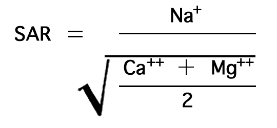
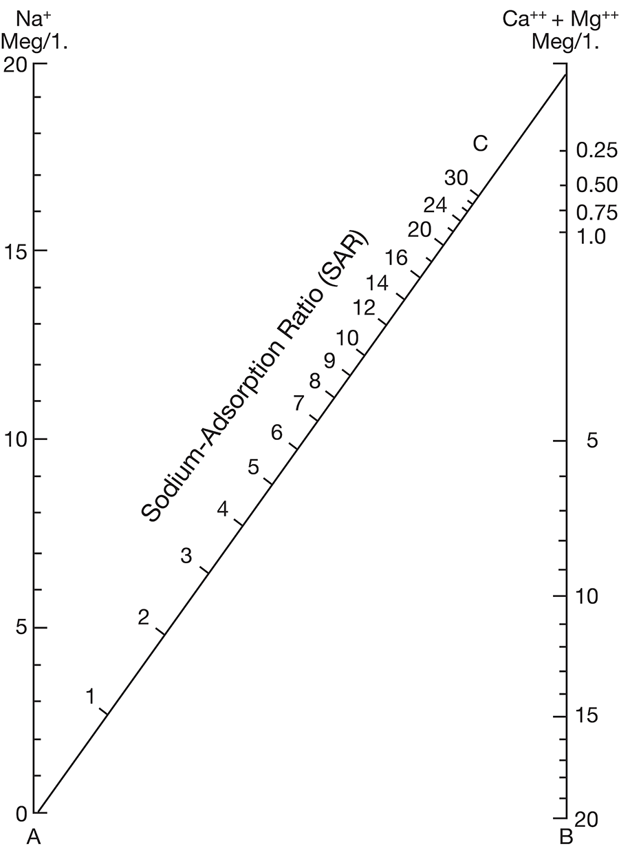
where the ionic concentrations are expressed in equivalents per million. The sodium-adsorption ratio may be determined also by use of the nomogram shown in Figure 10. In using the nomogram to determine the sodium-adsorption ratio of a water, the concentration of sodium expressed in equivalents per million is plotted on the left scale (A), and the concentration of calcium plus magnesium expressed in equivalents per million is plotted on the right scale (B). The point at which a line connecting these two points intersects the sodium-adsorption-ratio scale (C) indicates the sodium-adsorption ratio of the water.
Figure 10--Nomogram for determining sodium-adsorption ratio of irrigation water.
When the sodium-adsorption ratio and the electrical conductivity of a water are known, the suitability of the water for irrigation can be determined by plotting these values on the diagram shown in Figure 11. Low-sodium water (S1) can be used for irrigation on almost all soils with little danger of the development of harmful levels of exchangeable sodium. Medium-sodium water (S2) will present an appreciable sodium hazard in certain fine-textured soils, especially under low-leaching conditions. This water may be safely used on coarse-textured or organic soils having good permeability. High-sodium water (S3) may produce harmful levels of exchangeable sodium in most soils and will require special soil management such as good drainage, high leaching, and additions of organic matter. Very high sodium water (S4) is generally unsatisfactory for irrigation unless special action is taken, such as addition of gypsum to the soil.
Figure 11--Diagram showing classification of water in Clay County for irrigation use.
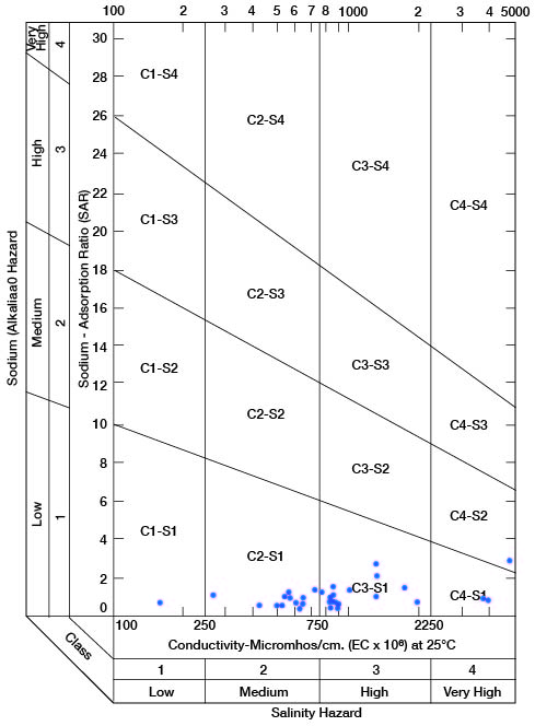
Low-salinity water (C1) can be used for irrigation of most crops on most soils with little likelihood that soil salinity will develop. Medium-salinity water (C2) can be used if a moderate amount of leaching occurs. Crops having moderate salt tolerances, such as potatoes, corn, wheat, oats, and alfalfa, can be irrigated with (C2) water without special practices. High-salinity water (C3) cannot be used on soils with restricted drainage. Very high salinity water (C4) can be used only on certain crops and then only if special practices are followed.
Boron is essential to normal plant growth, but the quantity required is very small. Crops vary greatly in their boron tolerances, but in general it may be said that the ordinary field crops common to Kansas are not adversely affected by boron concentrations of less than 1 ppm.
Prolonged use, under adverse conditions, of water having a high concentration of bicarbonate could have an undesirable effect upon the soil texture and plant growth.
Water samples (1 composite) from 33 wells and test holes are classified on Figure 11 to show the suitability of the water for irrigiation use. The wells or test holes corresponding to points shown in Figure 11 are given in Table 5. Of 32 samples of water from Clay County, 2 are of low alkali hazard and low salinity hazard and are very good irrigation waters; 7 analyses indicate a low alkali hazard and medium salinity hazard, and the waters are satisfactory for irrigation of most crops grown in Clay County; 20 samples represent water of low alkali hazard but high salinity hazard, but as most of these samples fall within the lower part of the high-salinity area, only moderate precautionary measures would be necessary. Three samples were of low or medium alkali hazard but very high salinity hazard, and such waters are unfit for irrigation use. In general, the aquifers in Clay County that produce water that is unfit for irrigation do not produce large enough quantities to be considered for irrigation.
Table 5--Sodium-adsorption ratios (SAR), conductivity (C), and class of water for irrigation for wells plotted on Figure 11. Composite sample from wells 7-4-20ad and 7-4-21bc.
| Well number |
SAR | C | Class |
|---|---|---|---|
| 6-1-2bac1 | 1.07 | 537 | S1-C2 |
| 6-1-2cc | .75 | 563 | S1-C2 |
| 6-1-15da | 1.21 | 573 | S1-C2 |
| 6-2-3ad | 1.80 | 892 | S1-C3 |
| 6-2-32ccc | .78 | 2,070 | S1-C3 |
| 6-2-33cd | .62 | 820 | S1-C3 |
| 6-4-18ba | .85 | 3,950 | S1-C4 |
| 6-4-33ad | .44 | 673 | S1-C2 |
| 7-1-6bb | 1.26 | 784 | S1-C3 |
| 7-1-15bcb | 2.16 | 1,330 | S1-C3 |
| 7-1-19bc | 1.8 | 272 | S1-C2 |
| 7-2-4ddc | .60 | 803 | S1-C3 |
| 7-3-4da | .60 | 3,970 | S1-C4 |
| 7-3-29cd | .69 | 896 | S1-C3 |
| *7-4-(20ad=21bc) | .68 | 926 | S1-C3 |
| 7-4-32cc | .52 | 887 | S1-C3 |
| 8-1-13ca | 0.82 | 1,370 | S1-C3 |
| 8-2-30dd | 1.56 | 1,780 | S1-C3 |
| 8-3-8db | .59 | 900 | S1-C3 |
| 8-3-35da2 | .47 | 515 | S1-C2 |
| 8-4-15dc | .65 | 906 | S1-C3 |
| 9-2-30bb | .65 | 90 | S1-C1 |
| 9-3-1cc | 1.00 | 853 | S1-C3 |
| 9-3-20bc | .61 | 626 | S1-C2 |
| 9-3-23cc | .37 | 635 | S1-C2 |
| 9-4-21aa | .83 | 579 | S1-C2 |
| 9-4-32adc | .58 | 434 | S1-C2 |
| 10-1-17dc1 | .70 | 186 | S1-C1 |
| 10-2-17cd1 | 2.72 | 5,620 | S2-C4 |
| 10-2-23bb | 1.58 | 743 | S1-C2 |
| 10-3-13ba | 1.65 | 1,040 | S1-C3 |
| 10-4-32aa | .75 | 667 | S1-C2 |
Hydrologic Properties of Water-bearing Materials
The quantity of water that a water-bearing formation will yield to wells depends upon the hydrologic properties of the material from which the wells produce. The two hydrologic properties of greatest significance are the coefficients of transmissibility (T) and storage (S) and are used in making quantitative estimates of water available in an aquifer and of future water-level decline that will result from continued pumping. Controlled aquifer tests in the field provide the data required to compute these coefficients.
The coefficient of transmissibility (T) may be defined as the number of gallons of water at the prevailing temperature that will move in 1 day through a vertical strip of the aquifer 1 foot wide, having a height equal to the full thickness of the aquifer, under a hydraulic gradient of 1 foot per foot, or it is the number of gallons of water that will move in 1 day through a cross-sectional area equal to the saturated thickness of the aquifer and 1 mile wide under a hydraulic gradient of 1 foot per mile. The coefficient of storage (S) may be defined as the change in volume of water stored per unit surface area of aquifer per unit change in head. Under water-table conditions the coefficient of storage (S) is practically the same as the specific yield of the aquifer.
The coefficient of permeability (P) of an aquifer is the discharge per unit of area per unit of hydraulic gradient. It may be measured in terms of the number of gallons of water a day, at 60° F., conducted laterally through each mile of aquifer under investigation (measured at right angles to the direction of flow) for each foot of thickness of the aquifer, and for each foot per mile of hydraulic gradient. The field coefficient of permeability (Pf) is the same except that it is measured at the prevailing temperatures of the water rather than at 60° F. The coefficient of permeability may be expressed by the formula Pf = (T / m) where Pf is the field coefficient of permeability, T is the coefficient of transmissibility, and m is the thickness of the aquifer, in feet.
Aquifer-test Determination of Transmissibility and Permeabrlity
The coefficients of transmissibility and permeability of the alluvium and terrace deposits in the Republican River valley in the vicinity of Clifton were determined by an aquifer test using well 6-1-2ac owned by Mr. F. Turner and operated by Mr. H. Rhodes. Values for the coefficient of transmissibility (T), storage (S), and permeability (P) were computed from the aquifer-test data by formulas developed by C. V. Theis and C. E. Jacob.
Theis Recovery Method of Determining Transmissibility
The recovery method of computing transmissibility (T) developed by Theis (1935) utilizes a series of measurements of the water level in a well after a period of pumping.
The Theis recovery formula is expressed as:
T = (264Q log10 t/t') / s'
in which T is the coefficient of transmissibility, in gallons per day per foot, Q is the pumping rate, in gallons a minute, t is the time since pumping started, in minutes, t' is the time since pumping stopped, in minutes, and s' is the residual drawdown in the pumped well, in feet, at time t'.
The residual drawdown (s') is computed by subtracting the static-water-level measurement from the depth-to-water measurements at time t' after pumping ceases.
The proper ratio of log10 t/t' to s' is determined graphically by plotting log10 t/t' on the logarithmic coordinate and s' on the arithmetic coordinate of semilogarithmic paper. If log10 t/t' is taken over one log cycle it will become unity. The formula may then be expressed as T = (264Q / Δs) where Δs is the difference in drawdown over one log cycle. In practice, water levels at time t' may be plotted and the residual drawdown need not be computed. Because the value of T is directly related to the slope of the line formed by plotting water level against t/t' the selection of the proper points on the plot to determine Δs is very important. Theoretically, the relation s' to t/t' should plot as a straight line that passes through the point where residual drawdown is 0 and where t/t' approaches unity. In unconsolidated deposits this is not always true, as the observed line is nearly always a curve and seldom passes through the point of origin. Generally the early points on the recovery curve are erratic and do not fall in a straight line. This may be due in part to head loss in the well or to the surge of the column of water, which falls back into the well after the pump is shut off. For this reason it would seem that the points on the curve corresponding to the late part of the recovery period would be the most reliable and should be used in determining Δs. For many aquifer tests the recovery data will not plot on a line that passes through the point where s' = 0 and will not plot in a straight line in the latter part of the recovery period, and it is difficult to establish a line that will determine Δs. If the latest data where t/t' approaches 1 do not fall on a straight line, they should not be used. If the earlier points fall on a straight line they should be used, but if there is an appreciable curve to the line almost any value can be obtained for Δs, and hence the value of T can be considerably in error.
Straight-line Graphical Method of Determining Transmissibility and Storage Coefficient
The Theis (1935) nonequilibrium formula requires the use of a "type curve" on which the test-data curve is superimposed to determine the coefficients of transmissibility and storage. Cooper and Jacob (1946) devised a straight-line graphical method that does not require the type curve to accomplish the same purposes. In this method the data are plotted on semilogarithmic paper, on which the plotted points should fall in a straight line. Three equations were devised for determination of coefficients of transmissibility and storage by a distance-drawdown graph, a time-drawdown graph, and a composite graph. In the distance-drawdown graph, drawdown is plotted on the arithmetic scale and distance of observation wells in feet from the pumped well is plotted on the logarithmic scale. The formulas for coefficients of transmissibility and storage are:
T = 264 Q / Δs and S = 0.3 Tt / r02
In the time-drawdown graph, drawdown is plotted on the arithmetic scale and time in days is plotted on the logarithmic scale. The formulas for coefficients of transmissibility and storage are:
T = 264 Q / Δs and S = 0.3 Tt0 / r2
In the composite drawdown graph, drawdown is plotted on the arithmetic scale and the value t/r2 is plotted on the logarithmic scale. In this method the plots of all observation wells should fall in a straight line. The formulas for coefficients of transmissibility and storage are:
T = 264 Q / Δs and S = 0.3 T × (t/r2)0
In the above formulas, the symbols are:
T = coefficient of transmissibility, in gallons per day per foot,
S = coefficient of storage,
Q = rate of discharge of pumped well, in gallons per minute,
Δs = drawdown over one log cycle,
t = time since pumping started, in days,
r = distance from pumped well, in feet,
t0 = value of t where drawdown = 0,
r0 = value of r where drawdown 0,
t/r2)0 = value of t/r2 where drawdown = 0,
Turner Aquifer Test
An aquifer test was made in the fall of 1955 in which well 6-1-2ac was used. This well yields water from late Wisconsinan terrace deposits in the valley of Republican River. The well is of gravel-wall construction and is 18 inches in diameter and 70 feet deep. Three observation wells, a, b, and c, were drilled in a line at distances of 25, 50, and 100 feet respectively from, the pumped, well. The well was pumped at a rate of 800 gpm from 9:25 a.m. until 9:55 a.m., when pumping stopped for a period of 45 minutes, owing to a power failure. Pumping was resumed at 10:40 a.m. and continued until 1:13 p.m. Water-level measurements made during the pumping period and values for t are given in Table 6.
Table 6--Water-level measurements made during pumping and recovery periods in well 6-1-2ac, and values for (t).
| Time | Time since pumping started, t, in minutes |
Depth to water, in feet |
|---|---|---|
| 9:20 a.m | Static water level | 22.21 |
| 9:25 a.m. | Pumping started | |
| 9:25:20 a.m. | 0.3 | 31.35 |
| 9:25:45 a.m. | .75 | 32.87 |
| 9:26:15 a.m. | 1.25 | 33.55 |
| 9:26:45 a.m. | 1.75 | 33.99 |
| 9:27:15 a.m. | 2.25 | 34.17 |
| 9:28 a.m. | 3 | 34.44 |
| 9:29 a.m. | 4 | 34.77 |
| 9:29:30 a.m. | 4.5 | 34.86 |
| 9:30 a.m. | 5 | 34.95 |
| 9:30:30 a.m. | 5.5 | 35.04 |
| 9:31 a.m. | 6 | 35.11 |
| 9:31:30 a.m. | 6.5 | 35.19 |
| 9:32 a.m. | 7 | 35.26 |
| 9:32:30 a.m. | 7.5 | 35.32 |
| 9:33 a.m. | 8 | 35.36 |
| 9:33:30 a.m. | 8.5 | 35.42 |
| 9:34 a.m. | 9 | 35.48 |
| 9:34:30 a.m. | 9.5 | 35.52 |
| 9:85 a.m. | 10 | 35.57 |
| 9:36 a.m. | 11 | 35.67 |
| 9:37 a.m. | 12 | 35.78 |
| 9:38 a.m. | 13 | 35.83 |
| 9:39 a.m. | 14 | 35.89 |
| 9:40 a.m. | 15 | 35.95 |
| 9:45 a.m. | 20 | 36.15 |
| 9:50 a.m. | 25 | 36.47 |
| 9:55 a.m. | Pump off (power failure) | |
| 10:39 a.m. | 22.98 | |
| 10:40 a.m. | Pumping started | |
| 10:40:30 a.m. | 75.5 | 33.87 |
| 10:41 a.m. | 76 | 34.77 |
| 10:41:30 a.m. | 76.5 | 35.16 |
| 10:42 a.m. | 77 | 35.42 |
| 10:42:30 a.m. | 77.5 | 35.67 |
| 10:43 a.m. | 78 | 35.81 |
| 10:44 a.m. | 79 | 36.00 |
| 10:44:30 a.m. | 79.5 | 36.10 |
| 10:45 a.m. | 80 | 36.20 |
| 10:45:30 a.m. | 80.5 | 36.29 |
| 10:46 a.m. | 81 | 36.38 |
| 10:46:30 a.m. | 81.5 | 36.44 |
| 10:47 a.m. | 82 | 36.52 |
| 10:47:30 a.m. | 82.5 | 36.57 |
| 10:48 a.m. | 83 | 36.66 |
| 10:48:30 a.m. | 83.5 | 36.70 |
| 10:49 a.m. | 84 | 36.74 |
| 10:49:30 a.m. | 84.5 | 36.78 |
| 10:50 a.m. | 85 | 36.83 |
| 10:50:30 a.m. | 85.5 | 36.87 |
| 10:51 a.m. | 86 | 36.90 |
| 10:51:30 a.m. | 86.5 | 36.93 |
| 10:52 a.m. | 87 | 36.95 |
| 10:52:30 a.m. | 87.5 | 36.97 |
| 10:53 a.m. | 88 | 37.00 |
| 10:53:30 a.m. | 88.5 | 37.01 |
| 10:54 a.m. | 89 | 37.03 |
| 10:54:30 a.m. | 89.5 | 37.06 |
| 10:55 a.m. | 90 | 37.09 |
| 10:57 a.m. | 92 | 37.16 |
| 10:59 a.m. | 94 | 37.23 |
| 11:02 a.m. | 97 | 37.35 |
| 11:05 a.m. | 100 | 37.48 |
| 11:10 a.m. | 105 | 37.61 |
| 11:15 a.m. | 110 | 37.78 |
| 11:20 a.m. | 115 | 37.90 |
| 11:25 a.m. | 120 | 38.00 |
| 11:30 a.m. | 125 | 38.13 |
| 11:35 a.m. | 130 | 38.22 |
| 11:40 a.m. | 135 | 38.30 |
| 11:50 a.m. | 140 | 38.48 |
| 12:00 noon | 155 | 38.55 |
| 12:10 p.m. | 165 | 38.60 |
| 12:20 p.m. | 175 | 38.67 |
| 12:30 p.m. | 185 | 38.81 |
| 12:40 p.m. | 195 | 38.86 |
| 12:50 p.m. | 205 | 38.90 |
| 1:00 p.m. | 215 | 38.94 |
| 1:10 p.m. | 225 | 38.96 |
| 1:13 p.m. | 228 Pump off | |
| 1:14 p.m. | 229 | 26.83 |
| 1:15 p.m. | 230 | 26.38 |
| 1:16 p.m. | 231 | 26.17 |
| 1:17 p.m. | 232 | 26.01 |
| 1:18 p.m. | 233 | 25.90 |
| 1:19 p.m. | 234 | 25.80 |
| 1:20 p.m. | 235 | 25.71 |
| 1:21 p.m. | 236 | 25.63 |
| 1:22 p.m. | 237 | 25.57 |
| 1:23 p.m. | 238 | 25.49 |
| 1:24 p.m. | 239 | 25.44 |
| 1:25 p.m. | 240 | 25.39 |
| 1:26 p.m. | 241 | 25.35 |
| 1:28 p.m. | 243 | 25.26 |
| 1:30 p.m. | 245 | 25.16 |
| 1:32 p.m. | 247 | 25.09 |
| 1:34 p.m. | 249 | 25.02 |
| 1:36 p.m. | 251 | 24.95 |
| 1:38 p.m. | 253 | 24.90 |
| 1:41 p.m. | 256 | 24.80 |
| 1:44 p.m. | 259 | 24.74 |
| 1:47 p.m. | 262 | 24.66 |
| 1:50 p.m. | 265 | 24.58 |
| 1:54 p.m. | 269 | 24.52 |
| 1:58 p.m. | 273 | 24.45 |
| 2:02 p.m. | 277 | 24.38 |
| 2:06 p.m. | 281 | 24.32 |
| 2:10 p.m. | 285 | 24.24 |
| 2:15 p.m. | 290 | 24.15 |
| 2:21 p.m. | 296 | 24.09 |
| 2:28 p.m. | 303 | 24.01 |
| 2:35 p.m. | 310 | 23.98 |
| 2:45 p.m. | 320 | 23.91 |
| 2:55 p.m. | 330 | 23.81 |
| 3:05 p.m. | 340 | 23.74 |
| 3:15 p.m. | 350 | 23.66 |
| 3:25 p.m. | 360 | 23.60 |
| 3:35 p.m. | 370 | 23.54 |
| 3:50 p.m. | 385 | 23.46 |
| 4:05 p.m. | 400 | 23.40 |
| 4:20 p.m. | 415 | 23.32 |
In Figure 12 the depth-to-water measurements in the pumped well are plotted against time since pumping started. A line drawn through these points gives a value for Δs of 2.18. Applying the Cooper-Jacob formula, T = [(264) (800)] / 2.18 = 97,000 gpd per foot.
Figure 12--Depth to water in well 6-1-2ac plotted against time since pumping started.
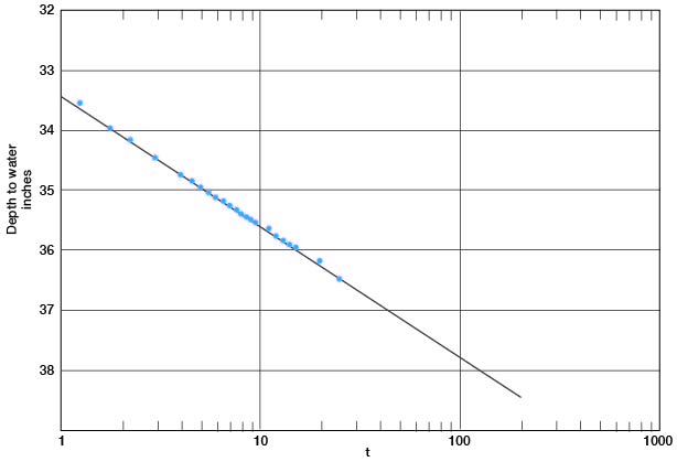
The saturated thickness is 43 feet, and from the relation P = T / m, P = 2,250. The pumped well had a drawdown of 17 feet while pumping 800 gpm; hence the specific capacity of the well was 47 gpm per foot of drawdown.
Depth-to-water measurements were made in observation wells a, b, and c during the test and are shown in Tables 7, 8, and 9.
Early in the test it was evident that observation well a was not responding to pumping as it should. The water-level measurements in Tables 7 and 8 indicate that the water level in observation well a was drawing down less than that in observation well b throughout the test. This was probably due to the lenticular nature of the aquifer rather than to any defect in the observation well, as tests made during the power failure indicated that the observation wells were open and functioning normally.
Table 7--Water-level measurements in observation well a, 25 feet from pumped well 6-1-2ac.
| Time | Time since pumping started, t, in minutes |
Depth to water, in feet |
|---|---|---|
| 9:20 a.m. | Static water level | 23.40 |
| 9:25 a.m. | Pumping started | |
| 9:26 a.m. | 1 | 24.31 |
| 9:27 a.m. | 2 | 24.69 |
| 9:29 a.m. | 4 | 25.05 |
| 9:30 a.m. | 5 | 25.23 |
| 9:32 a.m. | 7 | 25.56 |
| 9:34 a.m. | 9 | 25.72 |
| 9:36 a.m. | 11 | 25.93 |
| 9:38 a.m. | 13 | 26.08 |
| 9:40 a.m. | 16 | 26.23 |
| 9:42 a.m. | 17 | 26.33 |
| 9:44 a.m. | 19 | 26.47 |
| 9:46 a.m. | 21 | 26.60 |
| 9:48 a.m. | 23 | 26.69 |
| 9:50 a.m. | 25 | 26.78 |
| 9:53 a.m. | 28 | 26.98 |
| 9:55 a.m. | Pumping stopped | |
| 10:38 a.m. | 24.24 | |
| 10:40 a.m. | Pumping started | |
| 10:41 a.m. | 1 | 25.12 |
| 10:42 a.m. | 2 | 25.37 |
| 10:43 a.m. | 3 | 25.75 |
| 10:44 a.m. | 4 | 25.84 |
| 10:47 a.m. | 7 | 26.05 |
| 10:49 a.m. | 9 | 26.30 |
| 10:51 a.m. | 11 | 26.50 |
| 10:53 a.m. | 13 | 26.67 |
| 10:55 a.m. | 15 | 26.84 |
| 10:57 a.m. | 17 | 26.98 |
| 11:00 a.m. | 20 | 27.10 |
| 11:05 a.m. | 25 | 27.26 |
| 11:10 a.m. | 30 | 27.48 |
| 11:15 a.m. | 35 | 27.68 |
| 11:20 a.m. | 40 | 27.86 |
| 11:25 a.m. | 45 | 27.99 |
| 11:30 a.m. | 50 | 28.13 |
| 11:35 a.m. | 55 | 28.24 |
| 11:40 a.m. | 60 | 28.32 |
| 11:45 a.m. | 65 | 28.42 |
| 11:50 a.m. | 70 | 28.50 |
| 11:55 a.m. | 75 | 28.58 |
| 12:00 noon | 80 | 28.64 |
| 12:10 p.m | 90 | 28.69 |
| 12:20 p.m. | 100 | 28.80 |
| 12:30 p.m. | 110 | 28.89 |
| 12:30 p.m. | 120 | 28.98 |
| 12:50 p.m. | 130 | 29.03 |
| 1:00 p.m. | 140 | 29.09 |
| 1:10 p.m. | 150 | 29.15 |
Table 8--Water-level measurements in observation well b, 50 feet from pumped well 6-1-2ac.
| Time | Time since pumping started, t, in minutes |
Depth to water, in feet |
|
|---|---|---|---|
| 9:20 a.m | Static water level | 23.34 | |
| 9:25 a.m. | Pumping started | ||
| 9:26:30 a.m. | 1.5 | 26.63 | |
| 9:27:30 a.m. | 2.5 | 27.12 | |
| 9:28:15 a.m. | 3.25 | 27.32 | |
| 9:29 a.m. | 27.48 | ||
| 9:30 a.m. | 5 | 27.61 | |
| 9:31 a.m. | 6 | 27.71 | |
| 9:32 a.m. | 7 | 27.82 | |
| 9:33 a.m. | 8 | 27.90 | |
| 9:34 a.m. | 9 | 27.98 | |
| 9:35 a.m. | 10 | 28.04 | |
| 9:36 a.m. | 11 | 28.11 | |
| 9:38 a.m. | 13 | 28.19 | |
| 9:40 a.m. | 15 | 28.34 | |
| 9:42 a.m. | 17 | 28.43 | |
| 9:44 a.m. | 19 | 28.51 | |
| 9:46 a.m. | 21 | 28.59 | |
| 9:48 a.m. | 23 | 28.67 | |
| 9:50 a.m. | 25 | 28.75 | |
| 9:53 a.m. | 28 | 28.84 | |
| 9:54 a.m. | Pumping stopped | ||
| 10:38 a.m. | 24.00 | ||
| 10:40 a.m. | Pumping started | ||
| 10:41:30 a.m. | 1.5 | 76.5 | 27.48 |
| 10:43 a.m. | 3 | 78 | 27.98 |
| 10:44 a.m. | 4 | 79 | 28.22 |
| 10:45 a.m. | 5 | 80 | 28.36 |
| 10:46 a.m. | 6 | 81 | 28.47 |
| 10:48 a.m. | 8 | 83 | 28.84 |
| 10:50 a.m. | 10 | 85 | 28.89 |
| 10:52 a.m. | 12 | 87 | 28.90 |
| 10:55 a.m. | 15 | 90 | 29.04 |
| 10:58 a.m. | 18 | 93 | 29.15 |
| 11:00 a.m. | 20 | 95 | 29.23 |
| 11:05 a.m. | 25 | 100 | 29.38 |
| 11:10 a.m. | 30 | 105 | 29.51 |
| 11:15 a.m. | 35 | 110 | 29.66 |
| 11:20 a.m. | 40 | 115 | 29.77 |
| 11:25 a.m. | 45 | 120 | 29.85 |
| 11:30 a.m. | 50 | 125 | 29.95 |
| 11:40 a.m | 60 | 135 | 30.11 |
| 11:50 a.m. | 70 | 145 | 30.23 |
| 12:00 noon | 80 | 155 | 30.33 |
| 12:10 p.m | 90 | 165 | 30.45 |
| 12:20 p.m. | 1.00 | 175 | 30.54 |
| 12:30 p.m. | 110 | 185 | 30.63 |
| 12:40 p.m. | 120 | 195 | 30.69 |
| 12:50 p.m. | 130 | 205 | 30.73 |
| 1:00 p.m. | 140 | 215 | 30.79 |
Table 9--Water-level measurements in observation well c, 100 feet from pumped well 6-1-2ac.
| Time | Time since pumping started, t, in minutes |
Depth to water, in feet |
|---|---|---|
| 9:20 a.m | Static water level | 23.53 |
| 9:25 a.m. | Pumping started | |
| 9:26 a.m. | 1 | 23.57 |
| 9:27 a.m. | 2 | 23.64 |
| 9:28 a.m. | 3 | 23.73 |
| 9:29 a.m. | 4 | 23.81 |
| 9:30 a.m. | 5 | 23.88 |
| 9:31 a.m. | 6 | 23.97 |
| 9:32 a.m. | 7 | 24.04 |
| 9:33 a.m. | 8 | 24.12 |
| 9:34 a.m. | 9 | 24.18 |
| 9:35 a.m. | 10 | 24.24 |
| 9:36 a.m. | 11 | 24.31 |
| 9:37 a.m. | 12 | 24.38 |
| 9:38 a.m. | 13 | 24.44 |
| 9:39 a.m. | 14 | 24.50 |
| 9:40 a.m. | 15 | 24.56 |
| 9:42 a.m. | 17 | 24.66 |
| 9:44 a.m. | 19 | 24.78 |
| 9:46 a.m. | 21 | 24.90 |
| 9:48 a.m. | 23 | 25.00 |
| 9:50 a.m. | 25 | 25.09 |
| 9:53 a.m. | 28 | 25.21 |
| 9:54 a.m. | Pumping stopped | |
| 10:38 a.m. | 24.37 | |
| 10:40 a.m. | Pumping started | |
| 10:41 a.m. | 1 | 24.39 |
| 10:42 a.m. | 2 | 24.45 |
| 10:43 a.m. | 3 | 24.52 |
| 10:44 a.m. | 4 | 24.58 |
| 10:45 a.m. | 5 | 24.66 |
| 10:46 a.m. | 6 | 24.73 |
| 10:47 a.m. | 7 | 24.79 |
| 10:48 a.m. | 8 | 24.86 |
| 10:49 a.m. | 9 | 24.93 |
| 10:50 a.m. | 10 | 24.99 |
| 10:52 a.m. | 12 | 25.10 |
| 10:54 a.m. | 14 | 25.21 |
| 10:56 a.m. | 16 | 25.23 |
| 10:58 a.m. | 18 | 25.42 |
| 11:00 a.m. | 20 | 25.51 |
| 11:03 a.m. | 23 | 25.63 |
| 11:06 a.m. | 26 | 25.76 |
| 11:09 a.m. | 29 | 25.86 |
| 11:12 a.m | 32 | 26.00 |
| 11:15 a.m. | 35 | 26.09 |
| 11:20 a.m. | 40 | 26.25 |
| 11:25 a.m. | 45 | 26.38 |
| 11:30 a.m. | 50 | 26.52 |
| 11:35 a.m. | 55 | 26.62 |
| 11:40 a.m. | 60 | 26.71 |
| 11:45 a.m. | 65 | 26.94 |
| 11:50 a.m. | 70 | 26.95 |
| 11:55 a.m. | 75 | 27.02 |
| 12:00 noon | 80 | 27.07 |
| 12:10 p.m | 90 | 27.20 |
| 12:20 p.m. | 100 | 27.30 |
| 12:30 p.m. | 110 | 27.43 |
| 12:40 p.m. | 120 | 27.49 |
| 12:50 p.m. | 130 | 27.57 |
| 1:00 p.m. | 140 | 27.59 |
| 1:10 p.m. | 150 | 27.67 |
| 1:13 p.m. | Pumping stopped | |
| 1:14 p.m. | 1 | 27.62 |
| 1:15 p.m. | 2 | 27.58 |
| 1:16 p.m. | 3 | 27.53 |
| 1:17 p.m. | 4 | 27.45 |
| 1:18 p.m. | 5 | 27.42 |
| 1:19 p.m. | 6 | 27.39 |
| 1:20 p.m. | 7 | 27.29 |
| 1:21 p.m. | 8 | 27.28 |
| 1:22 p.m. | 9 | 27.22 |
| 1:23 p.m. | 10 | 27.17 |
| 1:24 p.m. | 11 | 27.13 |
| 1:25 p.m. | 12 | 27.09 |
| 1:26 p.m. | 13 | 27.05 |
| 1:27 p.m. | 14 | 27.01 |
| 1:28 p.m. | 15 | 26.97 |
| 1:29 p.m. | 16 | 26.93 |
| 1:30 p.m. | 17 | 26.88 |
| 1:31 p.m. | 18 | 26.86 |
| 1:32 p.m. | 19 | 26.83 |
| 1:33 p.m. | 20 | 26.78 |
| 1:34 p.m. | 21 | 26.76 |
| 1:35 p.m. | 22 | 26.73 |
| 1:36 p.m. | 23 | 26.69 |
| 1:37 p.m. | 24 | 26.67 |
| 1:38 p.m. | 25 | 26.64 |
| 1:40 p.m. | 27 | 26.58 |
| 1:45 p.m p.m. | 32 | 26.45 |
| 1:50 p.m. | 37 | 26.34 |
| 1:55 p.m. | 42 | 26.23 |
| 2:00 p.m. | 47 | 26.14 |
| 2:05 p.m. | 52 | 26.05 |
| 2:10 p.m. | 57 | 25.97 |
| 2:15 p.m. | 62 | 25.89 |
| 2:20 p.m. | 67 | 25.82 |
| 2:25 p.m. | 72 | 25.75 |
| 2:30 p.m. | 77 | 25.69 |
| 2:40 p.m. | 87 | 25.58 |
| 2:50 p.m. | 97 | 25.49 |
| 3:00 p.m. | 107 | 25.39 |
| 3:10 p.m. | 117 | 25.31 |
| 3:20 p.m. | 127 | 25.23 |
| 3:31 p.m. | 138 | 25.14 |
| 3:45 p.m. | 152 | 25.05 |
| 4:00 p.m. | 167 | 25.00 |
| 4:15 p.m. | 182 | 24.88 |
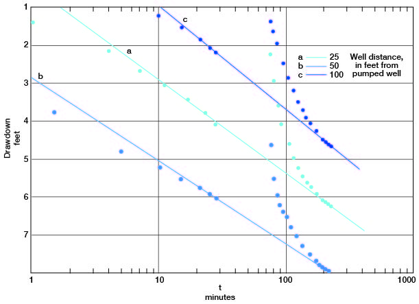
The drawdowns in observation wells a, b, and c are plotted against the time since pumping started (Fig. 13). Lines through the latest points prior to the power failure pass through the latest points in the test in all the plots. Applying the Cooper-Jacob formula, values for the coefficient of transmissibility from the fluctuations in observation wells a, b, and c are 87,000, 97,000, and 79,000 gpd per foot respectively. The storage coefficient, from measurements in wells a and c, was 0.03 and 0.02, respectively, indicating water-table conditions.
Figure 13--Drawdown in observation wells a, b, and c plotted against time since pumping started, during test using well 6-1-2ac.
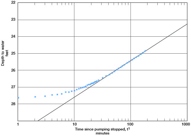
A line through the latest points in the recovery curve for well c (Fig. 14) gives a value for s = 2.17. Applying the formula
T = [(264) (800)] / 2.17
gives a result of 97,000 gpd/per foot.
Figure 14--Depth to water in observation well c plotted against time since pumping stopped, during test using well 6-1-2ac.
Summary--The values of T obtained from the aquifer test using well 6-1-2ac ranged from 79,000 to 97,000 gpd per foot. The lowest value was 79,000 gpd per foot from observation well a and the highest value, 97,000 gpd per foot, from the pumped well, observation well b, and the recovery curve for observation well c. The test is not conclusive, but 90,000 gpd per foot is probably about the correct value of T in the area of the well. The test shows that the aquifer is not homogeneous and that conditions are variable within short distances. The values for S are too small to have any significance, because of the shortness of the period of pumping.
Prev Page--Ground water recharge, discharge, utilization || Next Page--Rock units
Kansas Geological Survey, Geology
Placed on web April 7, 2009; originally published June 1959.
Comments to webadmin@kgs.ku.edu
The URL for this page is http://www.kgs.ku.edu/General/Geology/Clay/05_gw2.html