|
|
|
|
Progress Report on Intermediate Processing and Preliminary Interpretation of Baseline (November 2003) and the First Three Monitor 3-D Surveys (January, March, June 2004) |
|
|
|||
Processing data from each of the different surveys followed as near the same flow as possible, only changing parameters as necessary to accurately compensate for surface changes and equipment performance. No standardized equalization approach was used, the only changes unique to each survey were in response to variations in statics related to changes in soil conditions. A standard 3-D processing flow was used, minimizing applications that were influenced by data characteristics and focused on processes that act more uniformly on the different data sets. In general, the last four sweeps at each station were correlated, noise unique to each sweep removed, geometry assigned, and vertically stacked to provide the greatest signal-to-noise enhancement possible. These four-shot vertical stacks at each shot station were then muted to remove first arrivals, air-coupled wave, and ground roll. Prior to binning, these shot gathers were spectrally enhanced through deconvolution and digital filtering. Next the traces from each shot gather were sorted into their assigned bins, corrected to vertical incidence as a result of the different source-to-receiver offsets, and adjusted for trace-specific static irregularities. A variety of other processing operations were tested and some proved beneficial and will be used during final processing. Once the data were appropriately processed it was CMP stacked to produce a seismic volume.
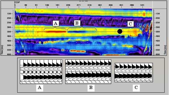
After production of a suitable seismic volume, any 2-D line can be extracted and viewed as a seismic cross section (Figure 1). In a 2-D format subtle differences in wavelet character can be recognized both horizontally (trace to trace) and vertically (as a function of depth). Since time-lapse techniques are being used on these data, subtle changes in wavelet characteristics are also readily recognizable over time (survey-to-survey). Changes appearing consistent throughout the time-depth interval on a single survey are likely related to the near surface. However, if changes are observed in reflection wavelets across a limited number of traces and within a small vertical time-depth window on different surveys, it is reasonable to suggest those changes are in response to variation in the rock properties somewhere within the subsurface volume. In some cases changes in seismic signature can be tracked to anomalous zones elsewhere in the section; shadow zones or dim outs are a common example.
Figure 1--A 2-D slice from the baseline survey during November 2003 with the approximate top of the Lansing-KC interval interpreted in red and an ellipse defining the area immediately below the L-KC appearing to change most dramatically when contrasted with the same 2-D cross line slice of the June 2004 survey. A larger version of this figure is available.
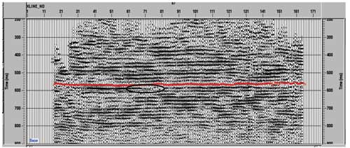
Comparing and contrasting 2-D cross line 87 from both the baseline and third monitor (June 2004) surveys, changes in seismic character are evident (Figures 1 and 2). Clearly with a dominant frequency of only around 60 Hz, much is still needed to enhance the higher frequency component of these data clearly present on shot gathers. However, even with this preliminary lower resolution data, a change in the reflection wavelet amplitude likely related to reflectivity and therefore the presence of CO2 is evident. This change in amplitude and wavelet character between the baseline and third monitor survey can be observed across a zone approximately centered beneath X-line 71 and near the top of what is interpreted as the Lansing-KC reflection at around 560 ms. This difference is quite pronounced considering that there has been no interval-specific processing done to these data specifically targeting the L-KC interval and this type of anomaly. Other changes in amplitude can be distinguished between the two surveys, but they are not consistent with theoretical expectation nor do they have a geometry that would lend itself to this kind of change in rock properties.
Figure 2--The same 2-D slice as Figure 1 except from the third monitor survey acquired in June 2004. As with the equivalent 2-D cross line slice, the approximate top of the Lansing-KC interval is interpreted in red with an ellipse defining a zone where a marked change in reflection character can be observed between the baseline and third monitor survey. A larger version of this figure is available.
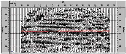
Careful study of differences between the two vertical slices through the seismic volume reveals other differences below the interpreted top of the Lansing-KC that are not directly related to the CO2 (there is some possibility that a few of these could be indirect indicators of changes in fluid properties). For example, differences such as beneath X-line 81 at about 650 to 700 ms appear different between the two data sets. However the depth of this anomalous zone beneath the L-KC (almost 100 ms) and its apparent isolation (that is, vertical connectivity as would be the case for a "shadow zone" related to increased attenuation or reflectivity due to the CO2) rule out this relative difference between the two surveys as related to the CO2 invasion. As well, intervals with differences in amplitude between the two surveys such as that visible between about 650 ms and 730 ms beneath station 111 are related to differences in source energy, coupling, cultural and natural noise, and other acquisition mismatches between the two surveys. Some data processing operations will effect slight changes in data characteristics unrelated to reservoir-specific change, as might be the case when noise levels change or soil conditions result in altered reflected wavelets.
In this thin layer pilot case study, it is essential to take into consideration that complex seismic responses to change in seismic velocity introduced by variations in pore fluid composition and therefore rock properties are similar to the apparent "velocity change" due to thickness change. Seismic modeling of a thinning layer (Figure 3) indicates that seismic amplitude may increase or decrease depending on whether thickness increases render layer thicknesses less than or greater than half the dominant seismic wavelength. We therefore took notice that the CO2-related amplitude dimming might be weakened or enforced by thickness related effects, depending on the region of thickness variability.
Figure 3a--Synthetic seismic for a thinning layer.
Figure 3b--Amplitude and Instantaneous frequency attributes variations with thickness in units of wavelength.
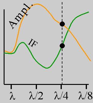
Figure 3c--Instantaneous frequency section of the thinning-layer synthetics and amplitude variations in time-window of the layer.
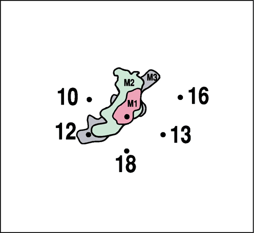
Nonuniform pore-fluid acoustic-property changes resulting from associated changes in reservoir pressures and facies within the pilot study area (pressure changes ranging from 11.7 - 106 N/m2 [1700 psi] at the injection well to 2.7 - 106 N/m2 [400 psi] near wells #12 and #13) and the associated continuum of CO2 proportions in the pore-fluid composition significantly complicate calculations of the effective pore-fluid properties, generalized over the entire flood-pattern. Consequently, we have attempted to get an approximate bulk snapshot of the effects of pore-fluid composition changes.
Gassmann's relations can be used to estimate rock-bulk modulus change for the two (effective fluid) pore-fluid compositions in proximity to the injection well. For our case, the two-fluid composition includes the combination of oil-water and miscible CO2-oil-water (Figure 4).
Figure 4--Gassman modeling. Percentage of property change equivalent to effective fluid (30% Oil+60% CO2 +10% Brine) compared to 100% (30%Oil+70%Brine) (pressure of 11 Mpa and temp. of 35°C).
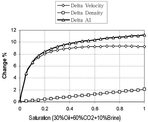
Unlike many carbonate reservoirs where significant facies changes can occur over very short distances, the relative lateral uniformity of petrophysical and lithological properties in the target oomoldic limestone interval should allow the use of Gassmann's type of fluid-replacement modeling. CO2-induced acoustic-impedance changes of up to 11% are expected based on these calculations.
Instantaneous frequency attributes provided a gross image of the aerial extent of the CO2 early in the program (previous web updates). With the need for horizon based interpretations and a higher resolution image of the CO2 plume as it expands across the site, a more detailed processing flow involving reflection specific enhancements and amplitude analysis was initiated. After the horizon interpreted as the L-KC "C" was identified on all 3-D seismic cubes (baseline and first 3 monitor surveys), the amplitude envelope attribute was calculated for the L-KC horizon. Amplitude envelope or reflection strength seismic attribute was selected because of it insensitivity to small phase shifts. This is especially important for this data set since the vibrator used for this study was not phase locked, minor variations in wavelet phase should be expected from survey to survey and shot to shot. Seismic reflection data for this study are all recorded uncorrelated, providing the opportunity during the later years of this study to apply phase compensation filters prior to correlation. This will allow defensible comparison of phase sensitive attributes in the future.
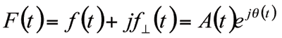
Amplitude envelope falls in the category of instantaneous attributes, which are based on the complex trace concept. A complex trace F(t) is given by:
Where f(t) = Real trace data, ![]() = Hilbert transform of real trace (quadrature trace),
= Hilbert transform of real trace (quadrature trace), 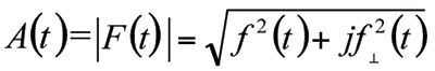 = Amplitude Envelope or reflection strength, and
 ![]() = Instantaneous phase. Those complex trace attributes provide instantaneous and quantitative description of seismic waveform.
= Instantaneous phase. Those complex trace attributes provide instantaneous and quantitative description of seismic waveform.
Average amplitude envelope is phase and frequency independent and more stable in terms of susceptibility to noise contamination when compared to many other seismic attributes. Those characteristics, besides the intrinsic property of being instantaneous, suggest that the average "median" amplitude envelope may be a robust candidate for time-lapse studies and enable a higher level of tolerance to imperfection in cross-equalization practices. For our application we used a "median value" of five samples around the time horizon. From analysis of synthetic examples, amplitude envelope has proven to be one of the most tolerant and robust properties to noise-effects and phase fluctuations.
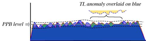
Considering the necessity to image a weak (in the vicinity of background noise) EOR-CO2 change, it was essential to apply an interpretation approach that avoided differencing time-lapse (TL) data or attribute with the corresponding baseline data or attribute. Our approach uses parallel progressive blanking (PPB), color balancing and color focusing of both baseline and TL amplitude envelope attribute and analysis of resulting textural differences (Figure 5). With the PPB method of interpretation, no differencing is applied; PPB is applied to both the baseline and the TL-amplitude envelope maps and a comparison/search for TL-textural reservoir signature is carried out. We applied the PPB method to balanced and normalized amplitude envelope maps of one baseline and three monitor amplitude envelope maps.
Figure 5--Schematic of the PPB approach of revealing below-background TL anomalies.
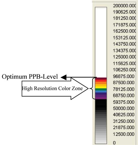
The PPB concept is based on the observation that differencing alone does not highlight reservoir anomalies if the change in magnitude of the seismic response is less than the amplitude of non-repeatable background noise. A background color is assigned to all values outside a narrow range within which the full color spectrum is focused to increase the sensitivity to fine details (Figure 6). In so doing, spatially significant textural differences can be enhanced at the highest level of resolution where otherwise the coarseness of the scale would have made these differences indistinguishable from noise. Using PPB, the sensitivity of the seismic signature to changes in the reservoir appears to be far greater than has previously demonstrated using more conventional approaches.
Figure 6--Sample color bar demonstrating how the fine sampled zone of data values can be presented in the highest resolution format possible.
The PPB approach can be illustrated (Figure 5) by placing a very weak TL attribute anomaly over a TL attribute profile from a seismically innocuous area (blue). Based on modeling, the expected change in amplitude from the incursion of CO2 is very low (below noise fluctuations). A textural interpretation approach is a much more effective way of distinguishing areas with such small changes in amplitude compared to differencing approaches (baseline survey [green] with a TL dataset [blue]). Delineating weak reservoir signatures by their textural characteristics is effective because of the inherent reduction in sensitivity to background noise and heighten resolution potential of the data.
For this seismic imaging program, PPB proved sensitive to weak time-lapse signatures that otherwise would have been concealed by noise and remnants of balancing/cross-equalization techniques. These textural differences are relatively stable over a range (two-three color steps) of scanned levels, suggesting their origin is production and/or EOR effects. These observations were verified with production simulation, production data, and consistency in multiple surveys.
As applied here, this newly developed 4D-seismic interpretation approach allows better focusing of color scales within the critical textural-difference range on time-lapse attribute maps, thereby enhancing apparent resolution within the critical range. Below the temporal resolution in thin heterogeneous stiff reservoirs, signatures of reservoir change are encoded in and interfered with by main events. Contribution of small changes in fluid saturation will manifest themselves as subtle spatial changes in texture rather than monotonically increasing or decreasing horizon attributes.
The PPB method is an alternative to TL-map differencing when targeting low S/N TL anomalies and can be described succinctly using the following expressions.
B(x,y) = St(x,y) + Nb,
where B(x,y) is the baseline survey attribute horizon map and a monitor survey (acquired at some later time) attribute horizon map
M1(x,y) = St(x,y) + Stl(x,y) + Nm,
where Nb and Nm are random noise in baseline attributes and TL attributes respectively, and Stl is the change in attributes due to a change in physical properties. The anomaly (Stl) is not distinguishable over the background signal/noise levels on difference maps (B-M1), when Nb - Nm is equal to or greater than STL. The extremely subtle STL imprinted on the ST, combined with the non-geologic, highly variable Nm results in textural differences between baseline and monitor horizon attributes at "optimum" PPB-level. This textural change is only observable when PPB-levels for the baseline horizon are selected near background levels. Intrinsic with this approach is the need to suppress background noise so a larger color range is available within this critical variability range of TL and baseline attribute maps.
With the expected small change in seismic response relative to the change in fluid during the CO2 flood at the Hall-Gurney field, the utilization of the PPB method for interpretation of the presence of CO2 is believed to provide accurate results (Figure 4). Since this method does not involve differencing, PPB can be applied to amplitude envelope maps of baseline and monitor data without equalization operations. Unlike differencing, PPB allows more control (determining the PPB range and scale segmentation) on the part of the interpreter, placing a more significant emphasis on matching display characteristics with the geologic setting.
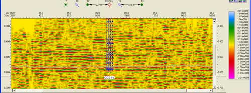
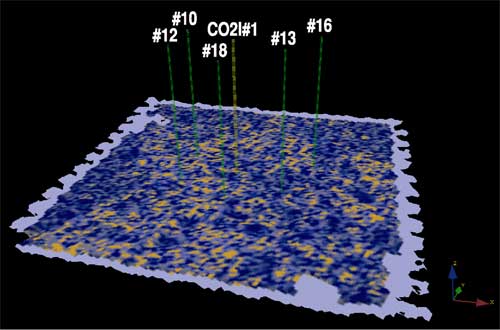
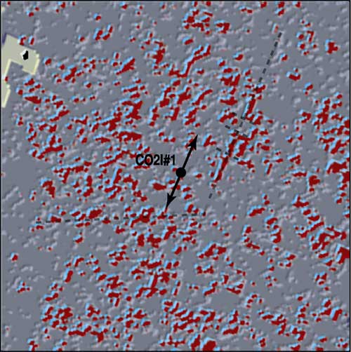
Most data were of good quality providing an excellent match between seismic cross-sections and synthetic traces (Figure 7). The target seismic horizon (gray) is at about 570 ms two-way travel time and for this project is defined as represented by a peak amplitude value.
Figure 7--Seismic amplitude section, interpreted target top horizon (gray), and seismic synthetics at well CO2I#1. Gas shadow effect is evident below time horizon in the vicinity of the injection well. A larger version of this figure is available.
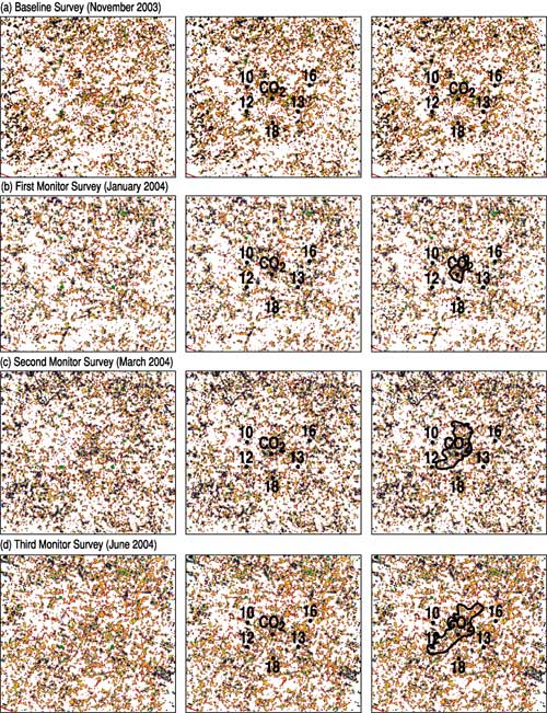
Expansion of the CO2 plume within the pilot area was successfully monitored seismically and tested against field production data (Figure 8a, b, c, d). Amplitude envelope attribute for the L-KC "C" was extracted from the horizon interpreted independently throughout each seismic volume. Synthetics generated from the sonic log of the CO2 injection well were a principal guide in consistently identifying the appropriate wavelet. Comparison of the four different amplitude envelope attribute maps of data acquired over an eight-month period clearly shows the subtle nature of the anomaly associated with the CO2 plume. However, using reasonable constraints on interpretations the affected area can be identified with reasonable confidence for each of the unique TL images.
Figure 8--Amplitude envelope horizon map of baseline in November 2003 (a), first monitor survey in January 2004 (b), second monitor survey in March 2004 (c), and third monitor survey in June 2004 (d). A larger version of this figure is available.
Flood pressure distribution and consequent CO2 movement are strongly influenced by the presence of boundaries interpreted to exist in the pilot region. These have been discussed in previous progress reports. Previous field performance and modeling had indicated the presence of a permeability barrier south of well #18. Seismic data clearly show the presence of an anomaly consistent with this production response. A N-S seismic anomaly has also been identified to the east of CO2I#1 and lying between CO2I#1 and #13. This is discussed below.
Due to the weak signal/background seismic response the boundary of the region identified as having CO2 is not precise or unique. Given that CO2 originates from a single location (CO2I#1), it is logical to assume that areas indicating consistent seismic response change, and interpreted to exhibit the presence of CO2, would be connected with the injection source and exhibit a continuous invasion path from any CO2-occupied area back to CO2I#1. Regions not exhibiting a continuous connection to CO2I#1, but that exhibit what might be interpreted as a change in seismic response and the presence of CO2, are assumed to not contain CO2 but are noted (Figure 8). For the most part, the anomalous seismic region interpreted as having CO2 has exhibited a continuous and contained shape through all the time surveys. To verify how the region identified as containing CO2 agreed with the material balance of CO2 volume injected, volumetric analysis based on total injected fluid and mapped reservoir properties was performed to determine the reservoir conditions necessary to obtain the interpreted CO2 plume size and distribution. Volumetric analysis indicates that insufficient CO2 has been injected to have CO2 sweep through the entire thickness of the L-KC "C" zone for the areas defined seismically. However, the interpreted areal extent of CO2 is consistent with a volumetric model where CO2 migration is restricted, in some portion of the flood area, to a thin (1-2 ft thick) higher-permeability interval within the "C" zone. This was premised on assumed three-phase relative permeability relationships. This model for L-KC "C" zone permeability distribution vertically is consistent with permeabilities observed in CO2I#1.
Production data are consistent with the interpreted change in the CO2 plume area. The January 2004 and March 2004 surveys are interpreted to indicate that the CO2 plume reached well #12 very near the time of the March 2004 survey. Production data recorded increases in CO2 concentration in well #12 in March 2004. The June 2004 survey interpretation indicates CO2 approaching well #13 but not reaching the well. Production data show traces of CO2 reaching well #13 in October 2004.
Seismic mapping of the progression of the CO2 plume away from the CO2I#1 injector provides a consistent picture of plume development. In addition, observed changes in the CO2 plume through time are consistent with changes in field injection and production rates (Figure 9).
Figure 9--Interpreted boundary of the CO2 plume based on the first three monitor surveys (January, March, June 2004). Note CO2 movement toward well #13 only began to occur between the March and June Surveys in response to increased water injection in well #7. Also note the northwest appendage evident on the March 2004 survey has receeded in response to the increased water injection in well #10.
It is unlikely the area of the reservoir involved in the flood has uniform rock properties considering the geology as interpreted from seismic and well data. Based on ooid shoal geometries, it is not unreasonable that the seismically interpreted boundaries represent shoal boundaries and a possible tidal channel on the east and therefore, potentially, restrictions to CO2 flow. Within the flood area vertical and horizontal changes in reservoir porosity and permeability within and between bedsets would be expected to result in non-uniform migration both horizontally and vertically. The interpreted bounding anomalies could be expected to influence areal pressure distribution and CO2 flow. Differences in permeability within bedsets could be anticipated to result in vertical differences in permeability, as observed in CO2I#1, and CO2 movement along thin higher-permeability intervals for the distance that the high-permeability bedset extends.
Monitor surveys were acquired at gradually increasing time intervals following the pre-CO2 injection or baseline survey, acquired in November 2003, with injection of CO2 starting December 2003. Seismic monitoring of CO2 movement began with the first monitor survey 6 weeks after starting injection (M1), followed by the second monitor survey about 12 weeks after start of CO2 injection (M2), then a third monitor survey at 26 weeks (M3), and fourth monitor 42 weeks after start of CO2 injection (M4; Figure 9).
Movement of CO2 is a function of injected CO2 volume and pressure in CO2I#1, injected water volumes and pressures in wells #10 and #18, the production rates and bottom hole pressures in wells #12 and #13, and the distribution of reservoir properties in the flood area. Expansion of the CO2 plume appears to be predominantly in a northeast/southwest direction (Figure 9). Some CO2 flooding to the north of CO2I#1 was modeled in reservoir simulations prior to initiation of the flood. However, the northward extent of the CO2 area defined by seismic response is greater than reservoir simulations predicted. This may reflect more focused CO2 movement than modeled due to several factors including: 1) restriction of movement to the east by the observed permeability barrier; 2) decreased pressure drop to the southeast toward well #13 due to the presence of the permeability barrier; 3) possible enhanced permeability to the north, as indicated by good reservoir properties in wells #8 and #1; 4) under-production early in the flood resulting in movement of CO2 away from producing wells; and 5) under-injection in well #10 for the actual reservoir properties compared with those modeled resulting in less containment to the north than modeled.
As expected, changes in injection and production rates impacted the movement of the CO2. An apparent recession of the CO2 plume between monitor surveysM2 and M3 in the northwest is consistent with the response expected from an increase in water injection rate in well #10 initiated during that time interval (Figure 9).
Seismically, trends in lithologic relationships may be observable on a lineament attribute map of the horizon interpreted as the L-KC "C" (Figures 10 and 11). A strong northeast/southwest series of lineaments are evident across the entire area. The most pronounced of these lineaments lies between CO2I#1 and well #13 and extends across the entire survey area. Another notable northeast/southwest trending lineament bounds the western edge of the pilot area. Also evident is a secondary trend of much smaller and more discontinuous lineaments with a more east northeast/west southwest trend. These are especially pronounced in the northern half of the survey area. The possibility was investigated that these lineaments are a processing artifact representing a byproduct of the receiver and shot lines orientation that after grid rotation during the binning process would have a bearing consistent with that rotation. The orientation of neither the primary nor secondary seismic lineaments are consistent with the 22° grid rotation. Therefore, these lineaments are interpreted to not represent artifacts of processing or acquisition.
Figure 10--Lineament attribute map. The principal trend is northeast/southwest with secondary trends oblique to the principal trend with an orientation around west-northwest by east-southeast. The principal trends can be traced across the survey area, while the secondary trends are much more discontinuous. A larger version of this figure is available.
Figure 11--Seismic lineament maps rotated and annotated with well locations. The main trend of lineaments, shown in gold, is NNE-SSW. A larger version of this figure is available.
A strong correlation exists between the preferential movement of the CO2 through this reservoir and features evident on the lineaments attribute map. Overlaying the lineament attribute map with the amplitude envelope attribute image provides added support for the suggestion that orientation of rock properties might be influencing fluid movement through this reservoir (Figure 12).
Figure 12--Amplitude envelope seismic attributes for each monitor survey--a) M1, b) M2, c) M3--overlain by the seismic lineament attribute map calculated from the baseline survey.
Of particular interest are the two lineaments that appear to be influencing the expansion of the CO2 plume at the time of the second 3-D survey (Figure 12b). A generally west-to-east lineament running immediately south of well #12, in conjunction with water injection in #18, can be interpreted to be diverting the southern most "tail" of the CO2 plume from northeast to southwest to move westerly. Under the pressures and fluid present along the southern edge of the CO2 plume at the time of this survey, this lineament might represent a change in permeability and therefore is effectively channeling the CO2 in more of a southwesterly direction. A second dominant lineament runs approximately northeast to southwest between CO2I#1 and well #13 and was previously identified on the lineament-only attribute map. At the time of the second survey the CO2 plume had only just contacted this lineament southeast of CO2I#1.
Clearly development of the CO2 plume is strongly influenced by features enhanced on the seismic lineament attribute maps (Figure 13). Comparing each interpreted amplitude envelope map for the three monitor surveys overlain by the lineament map it seems that growth of the CO2 plume is consistently influenced by several key lineaments it encounters through time and lateral expansion. The two dominant lineaments are easy to identify, but of particular importance are the apparent breaches in the "barrier" as defined by the northeast/southwest lineament. These offsets could represent pathways through this northeast/southwest barrier and would provide CO2 access to well #13.
Figure 13--Major lineaments that appear to be influencing fluid movement away from CO2I#1. A larger version of this figure is available.
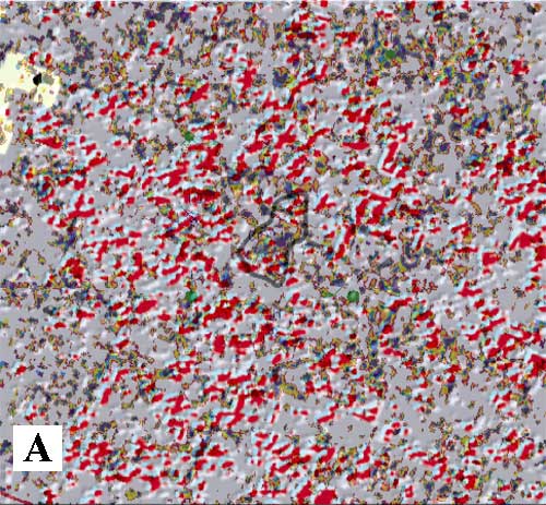
The similarity facies attribute map overlain by the L-KC horizon structure map provides a deeper look into possible lithologic explanations for the rate and path of the CO2 (Figure 14). From the facies map the northeast/southwest directionality of the lithology is evident. Detailed examination shows that the area near well #13 appears both topographically and lithologically different compared to the areas around wells #12 and CO2I#1. This difference may account for the delayed response of well #13.
Figure 14--Similarity "seismic facies" map on bottom of diagram. Highest similarity is shown in blue and lowest similarity shown in red. The better reservoir properties occur in blue areas as demonstrated by preferred (faster) EOR-fluid movement in those areas and generally in a SW-NE trend. Well No. 13 has had delayed response as a result of being separated from a CO2 injection well (yellow) by lower (golden-red) quality reservoir properties. The distribution and geometries associated with similarity seismic facies patterns are suggestive of a complex ooid shoal depositional motif, which is supported by oolitic lithofacies being the known reservoir in this interval (image approx. 0.75 mi. square). Upper map in diagram is a time structural map showing highest areas in red and lowest areas in blue. A larger version of this figure is available.
|
Kansas Geological Survey, 4-D Seismic Monitoring of CO2 Injection Project Placed online April 14, 2005 Comments to webadmin@kgs.ku.edu The URL is HTTP://www.kgs.ku.edu/Geophysics/4Dseismic/Process/Nov_2003/index.html |