Previous--Amplitude Variation with Offset || Next--Depositional and Stratigraphic Analysis of Kansas City Group Strata
1Kansas Geological Survey and 2Department of Geology and Geophysics, University of Missouri-Rolla
This article available as an Acrobat PDF file (5 Mb).
The interpreter who is used to conventional-resolution seismic data may be perplexed when confronted with high-resolution seismic data because conventional- and high-resolution data respond differently to the acoustic properties of the earth. For example, a high-amplitude, tuned, thin-bed reflection on a conventional seismic section may correspond to a low-amplitude, thick-bed event on a high-resolution section. Conversely, beds too thin to be effectively imaged by conventional data may be represented as high-amplitude, tuned reflections on high-resolution data. This may result in misidentification if the interpreter bases his stratigraphic correlations on amplitude response. Amplitude contrasts may also result from acoustic impedance gradients which generate high-amplitude reflections on conventional data but correspond to severely dimmed events on a high-resolution section. Lateral rugosity of the reflector surface and interference from adjacent thin layers can have a similar effect. As evidenced by models and seismic data incorporated into this paper, these factors result from the fact that conventional-resolution data and high-resolution data image different properties of the geologic strata.
Use of minimum-phase wavelets will cause time-correlation differences when data of different frequency content are compared and peaks or troughs rather than true wavelet onsets are picked. For this reason it is very important to ensure that data are processed to have zero-phase wavelets. Zero-phase wavelets also have the greatest resolving power; this is particularly important on high-resolution data. Because data of different frequency bands show different features of the earth, it may be advantageous in some situations to display each broad-band high-resolution section at a few different pass bands. Thus, features best imaged by conventional resolution are displayed and features best imaged by higher resolution are displayed.
Comparison of high-resolution data with conventional-resolution data and synthetic seismograms leads to inferences of vertical acoustic-impedance gradient and lateral surface rugosity. Vertical gradients on limestone surfaces, for example, may be related to porosity, and thus, recognition of their seismic signature may be an important interpretation tool.
High-resolution seismic data contain higher frequencies than conventional seismic section data but are not necessarily broader in terms of octaves of frequency bandwidth. Typically, seismic data contain two or three octaves of data. As Knapp (1990) points out, resolution of seismic data that contain at least a couple of octaves of frequency bandwidth is dependent on the values of the highest frequencies of the data. The limiting of octave bandwidth is a function of the logistics of seismic-data acquisition, attenuation by the earth, and instrument dynamic range. When recording high-resolution data, it is difficult to record low frequencies, or it is generally not done. Because the size of arrays is limited, low-frequency noise such as ground roll is often attenuated using frequency filters. Low-cut filtering and gain amplification are jointly applied to bring high frequencies within the dynamic range of the recording instruments. If low frequencies saturate the instruments, high frequencies can not be recorded (Knapp and Steeples, 1986). Conventional seismic data use long arrays to remove ground roll but are unable to record high frequencies because long arrays attenuate high frequencies. Also, high-power sources used in conventional data recording characteristically generate relatively longer wavelength (i.e., lower frequency) data. Because attenuation reduces the amplitude of the high-frequency data relative to the low-frequency data such that it is below the dynamic range of the instruments, it is important that the amplitude of high frequencies be maximized relative to that of the low frequencies. Conventional seismic data are generally looking deeper into the earth so that attenuation of high frequencies is more severe.
Significant differences are noticed between high-resolution sections and conventional sections recorded over identical geologic strata. Distinctive reflections on a highresolution section may be unnoticed on the low-resolution data because the beds are too thin for detection. This point is obvious because the objective of high-resolution is to image thin beds. Interestingly, however, prominent reflections on a conventional section may be severely muted on high-resolution data to the point where they may not be clearly identifiable. For instance, two limestones on a high-resolution section may have distinct reflection character differences, the thicker limestone being the one that is not well-imaged. There are several possible reasons for the differences. Most obvious is that on a seismic section, beds that correspond to tuning thickness will have the larger amplitude (Widess, 1973; Knapp, 1990). Tuning occurs when the thickness of the bed is approximately equal to one-fourth the apparent wavelength of the signal wavelet. Wavelength is equal to the interval velocity divided by the apparent frequency. Apparent frequency is the inverse of the time interval of one cycle (apparent period) of the wavelet. Tuning is constructive interference of the reflection from the base of a bed with the reflection from its top. Tuned thin beds on conventional data will be thick beds on high-frequency data. This will make a difference of perhaps a factor of two on the relative amplitude responses. But this factor does not account for all that is observed; there are two other possibilities.
High-resolution data, because they contain shorter wavelengths than conventional-resolution data, are more sensitive to vertical acoustic-impedance gradient and diffusive lateral rugosity of the reflection surface. Both of these factors cause a reduction of reflection amplitude. An acoustic-impedance gradient integrates the wavelet, causing a dispersion of the wavelet, lower frequency response, and lower amplitude response. It is possible that a reflector that has a strong response at low frequencies will be transparent to very high frequencies. Lateral rugosity causes a reduction in amplitude and/or dispersion of the wavelet, depending on mechanism of the rugosity. In fact, the response due to lateral rugosity can be identical to the response due to a vertical acoustic-impedance gradient. Without further information the two may be indistinguishable (Knapp, 1991). To distinguish the two, more geologic information is required; for instance, well logs will either confirm the gradient or not. If they do not, the inference is that the effect is due to lateral rugosity. Direct geological observation from outcrop or roadcut can also result in implications about reflection response. The misfortune is that frequently the two effects occur conjunctively. Unconformity surfaces are generally high-amplitude reflectors on conventional seismic data. Yet, by their nature, they generally have a weathered surface and are characterized by a velocity gradient. Generally, topographic highs exhibit more weathering. On the other hand lows may be infilled by detrital material. Thus, an unconformity may have both lateral rugosity and have a vertical gradient. This results in an even greater degree of amplitude reduction. Interference from adjacent interfering thin beds with lateral variation may also result in reduction of amplitude response. Vertical gradient may be related to porosity within carbonates. As such, recognition of the gradient may be useful as an exploration tool. A comparison of high-resolution data with conventional data or synthetic seismograms could help indicate the presence of a vertical velocity gradient.
Figure 1 shows the model response of a thin bed at different frequencies. At low frequencies (i.e., 25 Hz), the bed response is weak due to the destructive interference of the wavelet between the upper and the lower surfaces. For wavelets with long wavelengths, the positive reflection of the upper surface is partially masked by the negative reflection of the lower surface. At tuning (152 Hz), maximum amplitude response is seen. The trough from the upper positive reflection constructively interferes with the trough of the lower negative reflection. At high frequencies the response is that of a thick bed; the upper reflection and the lower reflection are separated by sufficient distance that the two reflections are effectively independent. The amplitude response of a thin bed can be nearly twice that of the response of a thick bed at high frequencies (i.e., 625 Hz) (Widess, 1973; Knapp, 1990).
Figure 1--Response of a bed of constant thickness at different frequencies. Layer thickness is 2.5 msec, corresponding to 5 m at 4,000 m/sec: (A) zero-phase wavelet, (B) minimum-phase wavelet.
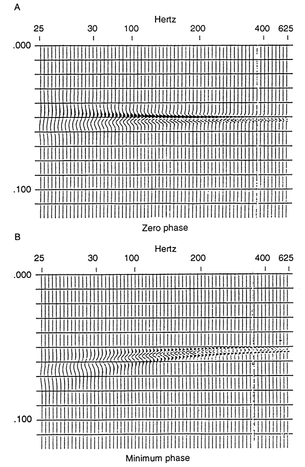
The implication from the thin-bed model is that peak amplitude response will occur when design of the frequency response of the seismogram corresponds to tuning of the bed. Thicker beds will be better resolved with low-frequency, conventional sections. Thinner beds will be better resolved with high-frequency, high-resolution sections. The stronger reflections seen on the conventional seismogram will appear as weaker reflectors on the high-resolution section. One who is used to conventional seismic sections and the characteristic amplitude of particular horizons may misidentify a thin-bed horizon on a high-resolution section because it appears to have an anomalous reflection response.
Figure 2 is the model response of a uniform acoustic-impedance gradient as a function of frequency. Low frequencies (i.e., 20 Hz) with wavelengths longer than the zone of the velocity gradient are not affected by the velocity gradient. Reflection response dims as a function of frequency (i.e., above about 100 Hz) as the wavelet is integrated. The wavelet is broadened and appears as a lower frequency event. Amplitude response is reduced. At high frequencies (i.e., above 160 Hz), the reflections within the zone cancel and only the edge residuals are seen, showing top and bottom of the zone as weak reflectors. Even these reflections dim with frequency. At very high frequencies (i.e., 625 Hz), the horizon is effectively transparent.
Figure 2--Response of a uniform acoustic-impedance gradlent as a function of frequency. The zone is 5 msec thick, corresponding to 10m at 4,000 m/sec: (A) zero-phase wavelet, (B) minimum-phase wavelet.
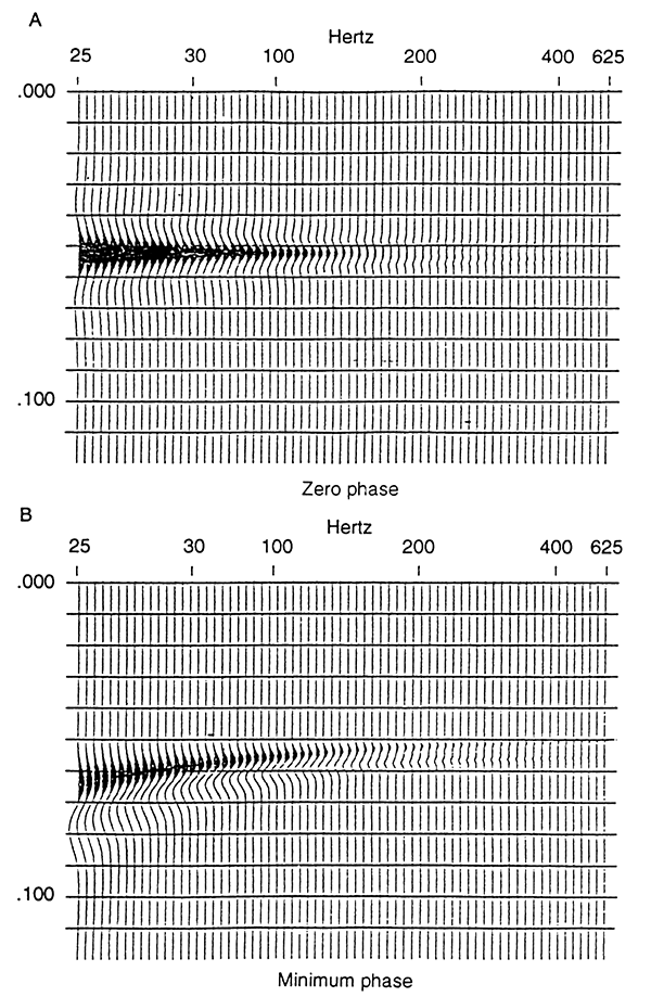
A reflector with a graduated top may be a strong reflector on a conventional section and a weak reflector on a high-resolution section because of the acoustic-impedance gradient. Again, the interpreter used to conventional sections may misidentify horizons or think that data quality is poor because a reflection known to be prominent on conventional data is weak or not detectable on the high-resolution section. This is a somewhat interesting paradox. The general intent of using a high-resolution survey is to image thinner and narrower targets. Yet the relative amplitude of the reflection of the target may be diminished by the nature of the target itself.
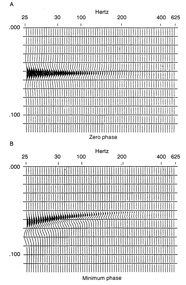
The effect of lateral rugosity depends on lateral resolution. Lateral resolution is dependent on a lateral wavelet (Berkhout, 1984; Claerbout, 1985). In addition to being sensitive to array size and the acoustic-impedance gradient of the earth, the lateral wavelet is dependent on frequency (Knapp, 1992). Thus, the higher frequencies (shorter wavelengths) of a high-resolution section are going to be more sensitive to lateral influences. A surface with short-wavelength, low-amplitude rugosity that may appear as a strong reflector on a conventional section may appear as a weak reflector on a highresolution section. Interestingly, the synthetic seismogram that is constructed from a well log will also show a high-amplitude event because it is one-dimensional and is not affected by lateral influences. This effect alone provides evidence of lateral rugosity. Because lateral wavelets are very broad, migration will not influence the resolution of short-wavelength rugosity.
Figure 3 shows the influence of lateral rugosity. By misfortune, the effect is nearly identical to that of an acoustic-impedance gradient when the rugosity is smoothed by the lateral wavelet (Knapp, 1991). Although use of arrays will aggravate the problem, they are not the sole source of the broad lateral wavelet, so use of single geophones is not the answer to the problem (see Data Examples).
Figure 3--Models of lateral rugosity as functions of frequency: (A) zero-phase wavelet, (B) minimum-phase wavelet.
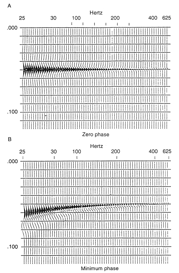
Interference from closely adjacent reflectors, such as sandstone channels, will also dim a reflection response because of interference. Although this effect exists on conventional seismic section, it will be aggravated on high-resolution section. The results are not necessarily dissimilar to the effects of lateral rugosity of the reflector surface except that channels may be large enough to be resolved and enhanced by migration. Figure 4 shows a section of a reflection response at different frequencies with channels present. The channel is modeled as an adjacent thin-bed reflector of reduced reflection coefficient. The effects of interference become more apparent as frequency increases. Dimming to 67% of the amplitude value at 25 Hz occurs between 200 and 300 Hz. Above 300 Hz, the presence of the thin layer becomes apparent in the response, and it amplifies in reflection strength as tuning begins to occur. Tuning frequency for the layer modeled is 1,000 Hz.
Figure 4--Model of interference from adjacent reflectors as a function of frequency: (A) zero-phase wavelet, (B) minimum-phase wavelet.
Because the interpreter tends to choose a peak or a trough as the arrival of the event, interpretational errors are possible (see fig. 1). Structure is apparent on both the zero-phase section and on the minimum-phase section, although the thin-bed reflector is flat. On zero-phase data, interference of a thin bed (at frequencies below the tuning frequency) pushes the dominant peak up at the top of the reflector, apparently creating a positive feature (see Knapp, 1990). The lower trough is forced downward. Apparent thickness is greater than the true thickness (Widess, 1973). Actual position of the reflector is in the middle of the response.
The minimum-phase response has similar problems. Although the top of the bed can be identified from the onset of the wavelet, picking of the peak places the top below its true position. The error exists at all frequencies but is reduced at higher frequencies.
Figure 2 shows similar problems for the velocity gradient model. For the zero-phase wavelet, the peak is in the middle of the gradient interval for frequencies less than 200 Hz, and does not correspond to either the top of the main bed or the base of the underlying gradient. Timing errors will either be positive or negative depending on what the interpreter chooses the peak to represent. The time position of the reflector is too great if the top of the interval is identified and too small if the top of the layer is identified. At frequencies greater than 200 Hz, it is the zero-crossing that corresponds to the boundaries of the interval. Picking of either the peak or the trough results in small timing errors.
Problems are even greater for the minimum-phase model. Onset of the wavelet does not correspond to either the top of the interval or its bottom, although the approximation gets better at high frequencies. At high frequencies a peak approximately corresponds to the onset of the gradient and a trough to its termination, but again, timing is in error, except at the highest frequencies. Picks on the conventional section results in the time being too great. Picking a peak rather than onset greatly accentuates the timing error.
In comparing seismic sections with different frequency characteristics, mis-ties will occur, especially if the sections are minimum-phase. This is because the peaks and troughs of minimum-phase arrivals are deeper than true-time position of the reflector. Further, as the models demonstrate, thin bed and velocity gradient intervals disperse the arrival to deeper depth, an occurrence that is more severe with low frequencies than high frequencies. Except for the thin-bed response, reflections of zero-phase wavelets will generally arrive on time. Thin-bed interference, however, will pull up a zero-phase wavelet when bed thickness is less than the tuning thickness.
In general, frequency response decreases with depth due to attenuation. This may result in mis-ties with a depth-to-time standard such as a velocity log. The problem is most severe in those cases where peaks or troughs are correlated on minimum-phase data. In this situation, the correlated deeper arrivals will be stretched in time, thus appearing to be too deep or leading to the conclusion that velocities are lower than true velocities. Thin beds and velocity gradients will also stretch the arrival downward. This effect will increase with decreasing frequency.
Zero-phase wavelets will result in correct timing regardless of frequency, except for the thin-bed situation where apparent pull-up will occur at frequencies less than tuning. The apparent pull-up will increase with decreasing frequency (fig. 1).
Figures 5 and 6 display a section of the upper Kansas City and Lansing Groups (Upper Pennsylvanian) with a velocity log from a nearby well and synthetic seismograms at several frequencies. The synthetic seismogram of fig. 5 with a 208-Hz Ricker wavelet suggests that the five limestones and four shales in the interval between South Bend and Farley limestones should be tuned, large-amplitude events on the highresolution section. However, this does not fit the observation on the data. The Springhill and Farley limestones are relatively weak reflectors on the seismic section. From roadcut observations, the Springhill is known to have lateral surface roughness (Knapp, 1991; Knapp and French, 1991). This causes reduction of the amplitude response as discussed and illustrated in fig. 3. Sandstone layers in the overlying Bonner Springs Shale destructively interfere with the Farley event. This reduces both the amplitude of the peak corresponding to the Farley Limestone and the trough corresponding to the Bonner Springs Shale (see fig. 4).
Figure 5--Upper Kansas City-Lansing, eastern Kansas, synthetic seismograms with different frequencies. The velocity log came from a well about 10 km from the seismic line (fig. 6).
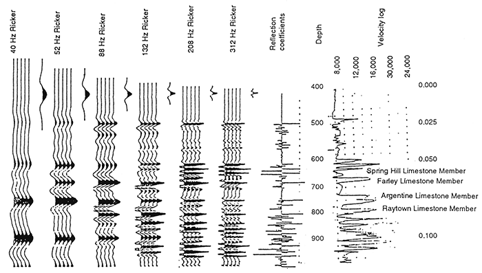
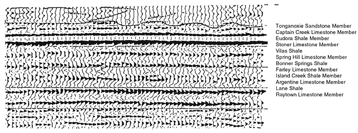
Figure 6--Seismic line highlighting Upper Kansas City-Lansing groups. The Southbend Limestone (Upper Pennsylvanian, Lansing Group), which is on the well log, has been at least partially eroded and replaced by the overlying Tonganoxie, a local channel sandstone.
The Argentine Limestone is dim on the seismic section (fig. 6) and shows lateral thickness variation and a reflector between the upper and lower units of the limestone bed. On the synthetic seismogram at high frequencies, it also appears to be a relatively low-amplitude event, because it is a thick bed and has split into two reflectors. At low frequencies it is a strong single reflector because its thickness tunes at between 50 and 90Hz.
Models and real data show that there are geologic situations that may cause conceptual difficulties for an interpreter experienced only with conventional-resolution, low-frequency seismic sections when high-resolution, high-frequency seismic sections are encountered. The situations are thin beds, acoustic-impedance gradient, lateral rugosity, and interference from adjacent thin layers. It is a paradox that the value of highresolution seismic data may be diminished in that high-amplitude, tuned reflections on a conventional seismic section will become low-amplitude, thick-bed reflections on a high-resolution section. In addition, acoustic-impedance gradients may dim an event which is manifested as a high-amplitude reflection on conventional data. Lateral rugosity and interference from adjacent layers can have a similar effect. Dimming can be so severe as to make the reflection transparent. In some cases all of these factors may be operating in conjunction; the fact is that high-resolution and conventional seismic data respond to different acoustic characteristics of the earth.
Thin-bed response can cause those horizons that generated strong, tuned reflections on conventional data to appear as relatively weak, thick-bed events on high-resolution data. This might cause the interpreter to misidentify a reflecting horizon. For example, a high-amplitude, thin-bed reflection on a conventional section could be miscorrelated with a high-amplitude, thin-bed reflection (of different origin) on high-resolution data. The Kansas City-Lansing example (figs. 5 and 6) illustrates such a case. The Wyandotte Limestone is a marker on the conventional section, and yet it is nearly transparent on the high-resolution data. However, other nearby reflectors, such as the contact between the Raytown Limestone and Liberty Memorial Shale, have a strong reflection response on the high-resolution section.
There are other situations which will cause amplitude dimming at higher frequencies. For example, an acoustic-impedance gradient may generate a high-amplitude reflection on a conventional section yet be transparent at high frequencies.
Lateral rugosity is sensitive to the frequency response of the data. At high frequencies, the dominant wavelength of the data approaches the dimensions of the rugosity and causes the reflection response to dim. The Springhill Limestone of the Lansing Group should be a medium-amplitude reflection according to the synthetic seismogram; however, as a result of surface roughness (diffusive rugosity), it is manifested as a weak event (figs. 5 and 6). The effects of rugosity can cause a response similar to that of a vertical acoustic-impedance gradient.
In the upper Kansas City Group, interference from thin sandstone layers in the Bonner Springs Shale causes dimming of the reflection response of the Farley Limestone (figs. 5 and 6). Without the sandstone layers, tuning would cause the Bonner Springs Shale and Farley Limestone to be a strong trough and peak combination. Instead, the trough has small reflectors representing the sandstone layers, reducing its amplitude, and the Farley Limestone is a relatively weak reflection.
Besides having lower resolution than zero-phase wavelets, minimum-phase wavelets cause frequency-dependent mis-ties of the data with depth in all the models shown. When that is coupled with the fact that frequency decreases with depth due to attenuation, this causes exaggeration of depth estimation, exaggeration of interval thickness, and underestimation of interval velocity.
Seismic-data acquisition is carefully designed to use sources of minimum energy, minimum noise, and maximum frequency and bandwidth. Pre-emphasis filtering helps balance the data spectrum during acquisition. Use of multiple geophones increases sensitivity which allows smaller and higher frequency sources to be used, reduces random noise according to the square root of the number of geophones, and attenuates air-coupled wave noise by judicious spacing. Array size is designed to be the maximum possible without adversely affecting frequency response at long offsets. Group-to-group distance is set to be equal to array size, and arrays are linear to fit the stack-array concept of Morse and Hildebrandt (1989). The stack-array, the use of half-integer source offset (Knapp, 1985), and split spread geometry help reduce ground roll when data are stacked during processing. Source design also helps reduce ground roll. Data are gathered to the farthest offset possible that will avoid wideangle reflections, and this is estimated to be about equal to the depth of the target reflector, but it is determined by field testing.
Wavelets are processed to be zero-phase or quadrature-phase because these phase designs have maximum resolving power and do not have the timing problems of other phase configurations (such as minimum-phase). Spectral whitening is used rather than deconvolution to balance the spectrum of the processed data because spiking deconvolution can adversely affect reflection character when the reflection coefficient series of the earth does not fit the presumption of randomness. Deconvolution, if used, is done judiciously and gently to remove specific problems such as multiples. Testing against synthetic seismograms can determine the degree of deconvolution that can be used without problems. Special care is taken in normal moveout, statics, residual normal moveout, residual statics, first arrival mutes, and mutes of normal moveout stretch to preserve the high-frequency quality of the field data and to show shallow reflections. For shallow data, moveout and stretch are particularly important because shallow data have more moveout than deeper data and the shallow section has a greater rate of change of velocity than the deeper part of the section.
Key reflectors can be shown at their greatest advantage by producing several sections with different pass bands. In this manner beds of different thicknesses can have a section with frequencies appropriate for tuning, creating maximum possible amplitude response and visibility, and characterizing bed thickness. Such sections would also indicate other features of the section such as acoustic-impedance gradients, lateral rugosity, and the presence adjacent of thin-bed interference.
Berkhout, A. J., 1974, Related properties of minimum-phase and zero-phase time functions: Geophysical Prospecting, v. 22, p. 683-709
Berkhout, A. J., 1984, Seismic resolution--a quantitative analysis of resolving power of acoustical echo techniques: Geophysical Press, Amsterdam, 228 p.
Claerbout, J. F., 1985, Imaging the earth's interior: Oxford and Boston, Blackwell Scientific Publications, 398 p.
Hunter, J. A., Pullan, S. E., Burns, R. A., Gagne, R. M., and Good, R. L., 1984, Shallow seismic reflection mapping of the overburden-bedrock interface with the engineering seismographSome simple techniques: Geophysics, v. 49, p. 1,381-1,385
Knapp, R. W., 1985, Using half-integer source offset with split spread data: The Leading Edge, v. 5, no. 1, p. 66-69
Knapp, R. W., 1990, Vertical resolution of thick beds, thin beds, and thin-bed cyclothems: Geophysics, v. 55, p. 1,183-1,190
Knapp, R. W., 1991, Effects of surface roughness or diffusivity on migration, and lateral and vertical resolution (expanded abstract): Proceeding of the 2nd International Congress of the Brazilian Geophysical Society, p. 863-865
Knapp, R. W., 1992, The size of a reflection point: Proceedings of the Canadian Society of Exploration Geophysicists, p. 95
Knapp, R. W., 1993, Energy distribution in wavelets and implications on resolving power: Geophysics, v. 58, no. 1, p. 39-46
Knapp, R. W., and French, J. A., 1991, Features in Kansas cyclothems seen by high-resolution seismology; in, Sedimentary modeling--Computer simulation and methods for improved parameter definition, E. K. Franseen, W. L. Watney, C. G. St. C. Kendall, and W. C. Ross, eds.: Kansas Geological Survey, Bulletin 233, p. 111-121 [available online]
Knapp, R. W., and Steeples, D. W., 1986, High-resolution common-depth-point reflection profiling-Field acquisition parameter design: Geophysics, v. 51, p. 283-294
Knapp, R. W., 1992, The size of a reflection point (abst.): Canadian Society of Exploration Geophysicists, Expanded Abstracts, p. 95
Morse, P. F., and Hildebrandt, G. F., 1989, Ground roll suppression by the stack-array: Geophysics, v. 54, p. 290-301
Widess, M. B., 1973, How thin is a thin bed?: Geophysics, v. 38, p. 1,176-1,180
Previous--Amplitude Variation with Offset || Next--Depositional and Stratigraphic Analysis of Kansas City Group Strata
Kansas Geological Survey
Comments to webadmin@kgs.ku.edu
Web version placed online Aug. 24, 2015. Original publication date 1995.
URL=http://www.kgs.ku.edu/Publications/Bulletins/237/Knapp2/index.html