Previous--Forward Seismic Modeling || Next--High-resolution and Conventional-resolution Seismic Data
1Kansas Geological Survey, 2Consultant, Wichita, and 3Department of Geology and Geophysics, University of Missouri-Rolla
This article available as an Acrobat PDF file (4 Mb).
Subsurface variation in the ratio compressional of P-wave velocity to shear (S-) wave velocity, Vp/Vs, yields an opportunity to observe amplitude variation with offset (AVO) effects. Ideally, such variations can be inverted to indicate lithology, porosity, constituent fluids, and/or presence of free gas. In practice, AVO techniques are somewhat limited by factors such as noisy data and actual subsurface materials.
One geological situation to which AVO techniques are ideally suited is the delineation of free gas-bearing sandstones. The dramatic decrease of Vp, relative to sandstone without gas, and the negligible change in Vs results in very large changes in Vp/Vs, i.e., Poisson's ratio. The AVO response is heavily dependent on that one parameter.
Data-quality control is critical with AVO measurements because many of the analyses are done with single trace common offset or CMP gathers, and measured amplitude response is very sensitive to noise. Data acquisition must include a large range of offsets, i.e., angles of incidence, ideally from 0 to 40°. A general rule of thumb is that far offsets need to be about 1.6 times the depth of the zone of interest. Recording of at least two components (vertical and radial) is desirable to rigorously derive true amplitude response of a P-wave reflection; however, the advantage of using a second component may not be truly cost-effective. Measured amplitude can be extremely accurate when corrected from offset information to an estimated true amplitude. Processing must maintain relative amplitude response of a reflection. This consideration affects and limits the use of AGC gain, deconvolution, and other space (trace) or time-adaptive processes. The display of AVO can be in the form of unstacked common offset gathers or CMP (CDP) gathers of instantaneous amplitude. Instantaneous amplitude compensates for phase-response differences on the peak amplitude of the reflection wavelet.
Individual traces on conventional, common midpoint (CMP)-stacked (equivalently, common depth point (CDP)-stacked) seismic data are assumed to be representative of zero-offset (normal incidence) reflections. For deep targets (depth ≥ far offset), the assumption is fairly accurate. Consequently, common analysis is frequently based on normal-incidence modeling, which is relatively straight-forward because zero-offset rays do not have mode conversion. A vertically incident P-wave generates only a reflected P-wave and a transmitted P-wave. The amplitude of the reflected wave depends on the reflection coefficient, and the amplitude of the transmitted wave depends on the transmission coefficient. The signs of the coefficients indicate polarity of the resultant modes, relative to the incident wave:
Reflection coefficient = (Zi + 1 - Zi)/(Zi + 1 + Zi)
= (1 - Zi/Zi + 1)/(1 + Zi/Zi + 1)
Transmission coefficient = 1 - R2
= 4(ZiZi + 1)/(Zi + Zi + 1)2
= 4(Zi/Zi + 1)/(1 + Zi/Zi + 1)2, (1)
where subscripts indicate the layer number from the surface, Z is acoustic impedance, the product of rock density, ρ, and rock velocity, V:
Z=ρV (2)
AVO techniques exploit the fact that the seismic amplitude response of a reflection (energy) is a function of its angle of incidence. Non-zero offset rays have mode conversion which splits the incident energy; a P-wave incident on an interface generates the following:
Figure 1--Mode conversion by incident P-Wave.
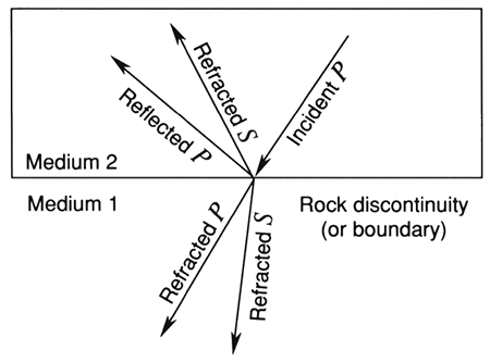
Mode conversion is a fact of the physics of continuous media that require conservation of energy and momentum, i.e., continuity of stress and strain, or continuity of vertical and tangential displacement, across the interface. A P-wave that reaches the interface at a non-zero incident angle has components at right angles to the direction of hypothetical transmission and reflection S-waves that set up the generation of shear (S-) wave energy in these directions. It also has components parallel to hypothetical transmitted and reflected P-waves that set up the generation of compressional (P-) wave energy in these directions. Thus, with offset (incident angle), varying amounts of P-wave energy are lost to the generation of S-waves and the splitting of P-wave energy into reflected and transmitted components.
The amplitude of a reflected P-wave varies with offset according to the reflection coefficient, which is dependent on acoustic-impedance contrast (ratio of the products of velocity and density), and Snell's Law, which is dependent on velocity contrast (velocity ratio).
In general, the product of velocity and density (acoustic impedance) is diagnostic of rock type; however, porosity complicates this value. One rock type at a particular porosity may have the same acoustic impedance as another rock type with different porosity.
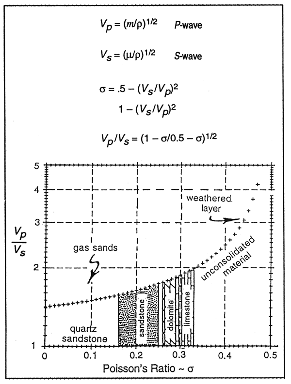
Seismic velocities depend on the square root of a modulus divided by density:
P-wave velocity is related to the modulus of confined extension, m:
Vp = [m/ρ]1/2 (3A)
S-wave velocity is related to only the shear modulus μ, and density ρ:
Vs = [μ/ρ]l/2. (3B)
The modulus of confined extension, m, is similar in concept to Young's modulus E, the modulus of unconfined extension. Both describe extension of a body due to tensile strain. In an unconfined body, lateral constriction is permitted. In a confined body, it is not.
Confined extension is related to unconfined extension E by Poisson's ratio σ:
m = E (1 - σ)/[(1 - 2σ)(1 + σ)] (4A)
= E (1.025 + 2σ2) + 2% (4B)
Confined extension differs from unconfined extension by 10 to 40% (σ = 0.20-0.40, respectively). As materials get more rigid, relative to compressibility, i.e., lower values of σ, confined extension and unconfined extension become closer in value. (For σ = 0, the two are equal.)
One of the more common equations for m is:
m = k + 4/3m. (5)
Thus,
Vp/Vs = [k/m + 4/3]1/2. (6)
where k is the bulk modulus.
Further, Poisson's ratio relates directly to Vp/Vs through the equation
σ = .5 - (Vs/Vp)2/1 - (Vs/Vp)2 (7)
Poisson's ratio a comes into play because it is dependent on the ratio Vp/Vs and, like density ρ, is relatively stable at depth under most circumstances. The two vary only slightly with rock type; in general, for sedimentary rocks, 0.3 < σ > 0.4 (σ ~ 0.35) and 2.2 < ρ > 2.7 (ρ ~ 2.5). Knowing or estimating constant values of σ and ρ, the first-order solution of the Zoeppritz (1919) equations is dependent only on the velocity ratio across the interface.
However, considering higher-order solutions of the Zoeppritz equations, AVO responses are theoretically sensitive to rock type. This is because the ratio of P-wave velocity to S-wave velocity, Vp/Vs, and σ are sensitive to lithology (fig. 2).
Figure 2-(A) Synthetic gas sand model. (B) Computed apparent reflection coefficient as a function of offset angle (Ostrander, 1984).
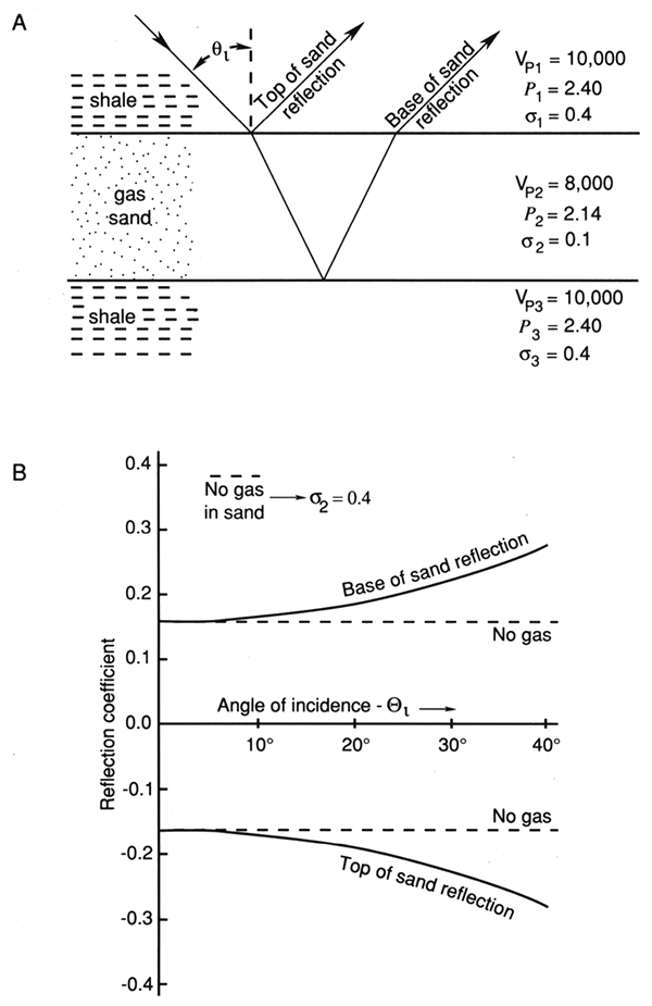
Vp/Vs measures the ratio of bulk modulus (incompressibility) to shear modulus. This can be a very subtle measurement and therefore difficult to derive by AVO methods. On the other hand, presence of gas in a reservoir causes a sufficiently dramatic contrast in the value of σi/σi + 1 that it may be practical to detect gas directly from AVO measurements. The presence of gas in a sandstone dramatically affects Vp but affects Vs only negligibly. Values of a may change from between 0.3 and 0.4 in the overlying rock to about 0.1 in the gas sand. The ratio σ1:σ2 may be as great as 3:1 or 4:1. In general, in the absence of gas, amplitude decreases very slightly with offset; however, in the presence of gas, the strong contrast in Poisson's ratio can cause amplitude to increase by more than 50% as angle of incidence increases from 0° to 30° or 40° (Ostrander, 1984). It is a radical change such as this that makes the use of AVO a viable diagnostic tool to determine the presence of gas. Figure 3 is a cross plot of Vp/Vs and ρ.
Figure 3--Cross plot of Vp/Vs and ρ.
Knapp (1977) determined Poisson's ratio values of near 0.45 (Vp/Vs = 3.32, k/m = 10) for very shallow consolidated carbonates, about 0.4 (Vp/Vs = 2.5, k/m = 5) for the deeper portions of the shallow cyclothemic carbonate-shale section of southern Indiana, and 0.33 (Vp/Vs = 2.0, k/m = 2.67) for the Cambrian-Ordovician Simpson Sandstone. The values are consistent with the interval transit time ratio ts/tp seen on P-wave and S-wave reflection seismograms (Tatham, 1992).
King (1966), measuring sandstones at 5,000 psi pressure [equivalent to 3,000 m (9,999 ft) depth] and porosity varying from 19 to 25%, determined values of Vp/Vs [s] from 1.65 [0.32] to 1.77 [0.36] when filled with a salt solution (median value .71 [0.35]); 1.55 [0.27] to 1.69 [0.34] with kerosene in the pores (median value 1.6 [0.30], and bimodal values of 1.51 [0.23] and 1.58 [0.29] when dry (1.55 [0.27] average).
Poisson's ratio values for the Green River Shale have been determined to vary between 0.22 and 0.30 (Podio et al., 1968). Hamilton (1976) measured Poisson's ratios of 0.45 to 0.50 for shallow marine sediments, with values decreasing with depth [600 m (2,000 ft) maximum depth]. For consolidated sediments, Gregory (1976) determined Poisson's ratio values of 0.20 to 0.30 when brine saturated and 0.20 to 0.14 when gas saturated. Domenico (1976 and 1977) determined values of about 0.40 for both unconsolidated sands and glass beads (38% porosity) when brine saturated and 0.10 when gas saturated.
Angle of incidence qi can be estimated from source-receiver offset X and reflector depth H using a simple straight ray-path assumption:
qi = tan-1(X/2H). (8)
This assumes that velocity does not substantially change with depth. Using Equation 5, the maximum angle of incidence is 26.6° when using the rule of thumb that maximum offset be equal to target depth. If velocity increases with depth, which generally is the case, angle of incidence will be under-estimated by source-receiver offset (Ostrander, 1984).
A better assumption is that velocity increases linearly with depth:
Vp = V0 + ΔV/δH · H H (9)
where ΔV/δH, the rate of increase with depth, can be measured from sonic logs or estimated from stacking velocity. The equation for angle of incidence qi versus offset X is:
qi=tan-1 {(HX+V0X/k)/(H2+2V0H/k-X2/4)}, (10)
where k = ΔV/δH.
Using the example of Ostrander (1984), Vp = 1800 + 0.6 H m/sec, the angle of incidence is 34° when H = X = 2,100 m (6,889 ft), Vp = 3,060 m/sec at H = 2,100 m (6,889 ft).
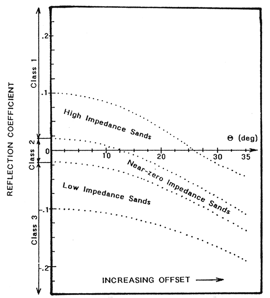
Rutherford and Williams (1989) developed a useful working classification of gas sands which distinguishes on the basis of encasing materials and hence reflection coefficients which will be generated at various offsets (incident angle). Figure 4 summarizes sands as follows:
In the example cited, Poisson's ratio and density for the gas sand were 0.15 and 2.0 g/cm3, respectively; those for the shale were 0.38 and 2.4 g/cm3. Note that in this case, Class 1 sands have a positive reflection coefficient (amplitude) until offset angle exceeds 25°. Class 2 sands can have positive amplitudes out to about 12°, but generally have negative coefficients; Class 3 sands have clearly negative amplitudes throughout.
Figure 4--Classification of gas sands, based on reflection coefficient variation with offset (angle of incidence) as proposed by Rutherford and Williams, 1989. Midcontinent sands (Cherokee, Morrow) will tend to be Class 1, where phase reversal occurs at longer offsets.
Many acquisition-design considerations for AVO and conventional CMP reflection data are similar. One main difference is that AVO data are considered best when recorded by at least two components (vertical and radial), so that true amplitude of the reflection can be determined. However, true amplitude can be estimated from a single vertical component by using angle of incidence:
Aest = Ameas/cos qi. (11)
The accuracy of the estimate depends on the accuracy of qi. The measurement of qi is very insensitive to errors in the estimate of V0 and fairly insensitive to errors in ΔV/δH. With 10% uncertainties in the estimates of V0 and ΔV/δH, errors are generally within ±2%. With such low sensitivity, increased accuracy achieved by using a radial component, if indeed there is any increase, is probably not worth the increased cost of acquiring and processing a second component of data.
Another primary difference is that all possible care must be taken to minimize noise so that AVO analysis can be done with single, unstacked traces and a minimum of enhancement processing. It is also more important that maximum offset be large so that reflections with large angles of incidence are recorded. Minimum offset should be as small as possible, yet large enough to avoid adverse interference from the source. Surface sampling should always be designed such that equal sampling of both the surface and the subsurface is maintained by the geophones for all gathers of the data: common source (field recorder order), common receiver, common offset, and common midpoint (CMP).
The best configuration geometry is split-spread, half-integer offset (shooting between the gaps) (Knapp, 1985) with shots at every interval. Geophone and source arrays should be linear, equally weighted, and equal in length to the group interval. Alternatively, when using a point source, the receiver array can be linearly tapered and equal in length to twice the group interval (see Knapp, 1992). These configurations automatically satisfy sampling requirements. Other configurations, split-spread integer offset (shooting on gaps) and end-on, also require such array design; however, to have the subsurface evenly sampled in a CMP gather requires two-trace mixing of the data during processing (i.e., stack array processing, Morse and Hildebrandt, 1989).
Array length is designed to be as long as possible without adversely affecting high-frequency response at far offsets. This means that array length for a linear, equally weighted array should be less than V/fmax. Linearly tapered arrays are the autoconvolution of a linear, equally weighted array, the response when both source and geophones have the same linear array design. The length of a tapered array should be equal to two times that of the linear array. Array length is not deliberately designed to attenuate ground roll noise, although attenuation of high-frequency ground roll is a consequence of array application. Low-frequency ground roll noise is attenuated by use of low-cut frequency filtering. Group interval is designed to be equal to array length, or, if a sufficient number of channels is available, equal to 1/n times the array length, where n is an integer.
Processing must be designed to maintain relative amplitude response laterally or, more exactly, down the normal moveout curves. Although this does not preclude the use of automatic gain control (AGC), the same function must be applied such that the gain applied to particular reflections is the same at all offsets. Use of deconvolution and other space or time adaptive processes have similar restrictions.
Data smoothing can help improve the accuracy of the measurement, but when overdone, it will change and smear the values. Such smoothing includes high-cut frequency filtering, trace-to-trace mixing of data in the CMP gather, record-to-record mixing of CMP gathers, and frequency-wave number filtering, a combination of all of the above. Judicious use of filtering may help reduce noise interference, but use of adaptive filters must maintain true relative amplitude response. Lateral mixing and wave number filtering of CMP records or common offset traces smear data spatially. This smearing must be very small with respect to lateral resolution. Lateral resolution can be estimated as the product of the vertical wavelet length in time and interval velocity of the target. Note that, contrary to common thought, lateral resolution is not related to Fresnel zone size (Knapp, 1991; Knapp, 1993). Mixing of CMP traces or common offset records smooths noise out of the measurement but must be small compared to the second derivative of AVO. Normal moveout correction is not done to avoid dispersion of the reflection by NMO stretch. Lateral alignment of a reflection is accomplished by a static shift.
An AVO display should be of instantaneous amplitude (square root of instantaneous energy) so that trace-to-trace phase differences within the wavelets does not influence measurement (Knapp, 1993). Polarity is determined from standard wiggle trace data, using CMP stacked data. Common offset (common incidence angle) displays are commonly most useful to make measurements. The alternative is to display unstacked CMP gathers.
While AVO responses can occur in a wide variety of rock types, current trends in application and research tend to be weighted toward sandstone reservoirs. This trend may evolve to include a greater emphasis on carbonate reservoirs, but the evidence presented here will be isolated to sandstones.
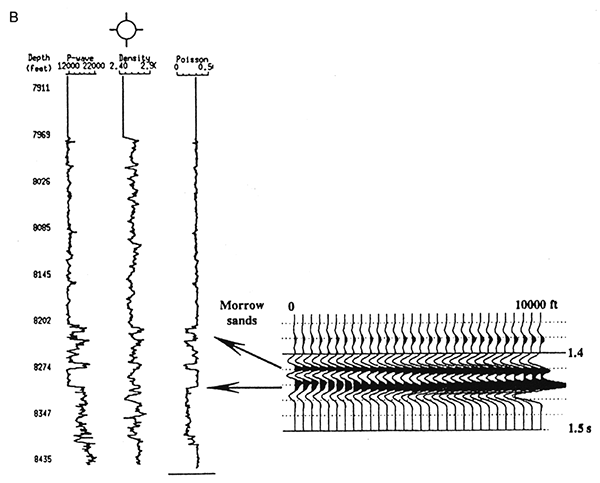
Figure 5, modified from Peddy et al. (1995), demonstrates how quick-look models can be generated to test anticipated AVO response from a Morrow sequence at a depth of about 8,300 ft. Utilizing sonic and density log control and applying an estimate for shear (S-) wave velocity, which then yields a Poisson ratio curve, synthetic offset seismograms have been generated using a filter representative of their data. The two comparison models relate two changing phenomena. The offset seismogram on the left represents response from a gas sand, occurring at a time of 1.430 sec; the seismogram on the right represents a similar sequence, but with wet brine sand in place of gas sand. Note also that the wet sand model also reaches longer offsets, 10,000 ft as opposed to 6,820 ft for the gas sand.
Figure 5A--Offset synthetic seismogram (CMP gather) demonstrating amplitude variation of gas sand at T = 1.430 sec. Note that P-wave velocity of Morrow sands is higher than overlying Morrow shale, while densities are nearly the same. Poisson's ratio of gas sand set at 0.15 for shale and Chester limestone ratio is set at about 0.35. Class 1 sand, based on Rutherford, 1989. Note offset range is 0-6,820 ft (2,046 m); sand depth is approximately 8,300 ft (2,490 m). Amplitude response of gas sand goes through complete phase reversal. (Modified from Peddy et al., 1995.)
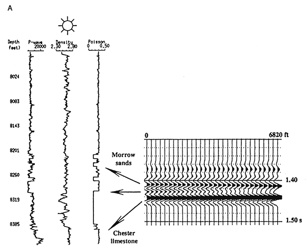
Figure 5B--Wet sand parameters substituted for gas sand in adjacent figure. Three thin sands interfere to produce a peak with an unchanging-to-slightly increasing AVO response at t = 1.430 sec. Chester limestone response is not included in this display. Note offset range is 0-10,000 ft (0-3,000 m). (Modified from Peddy et al., 1995.)
The theoretical AVO response in the gas sand synthetic is evident as a peak amplitude event at 1.430 sec, which eventually diminishes and finally reverses polarity at an offset of about 5,000 ft. In contrast, the wet sand never generates a truly discernible event which would likely be AVO anomalous.
The real data example in fig. 6 demonstrates in significant detail that the theoretical response is well represented in the Morrow sand zone at about 1.430 sec. The panels shown here have been extracted from the processed data volume in a variety of offset ranges; each panel represents a set of trace gathers in close proximity to the known gas sand. This is a clear-cut case of a Class 1 sand.
Figure 6--Actual data verifying predicted model response for gas sand at 1.430 sec. The reflection from the Morrow sand diminishes rapidly with increasing offset. Panels taken represent nearby CMP gathers. In each case, offset increases to the right. (Modified from Peddy et al., 1995.)
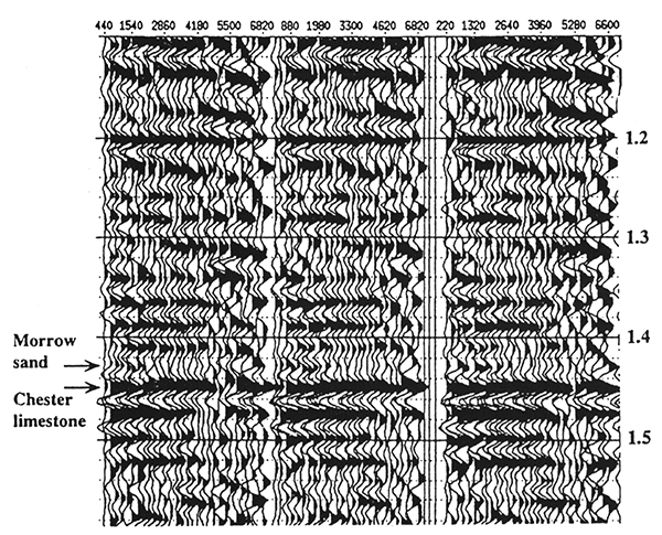
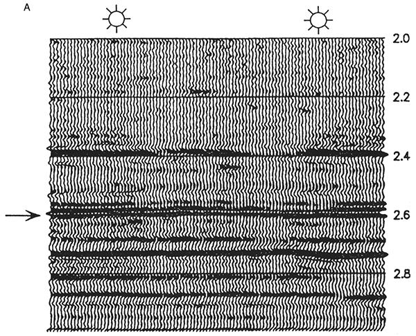
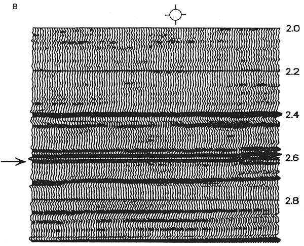
Figure 7 demonstrates a very strong AVO response in a stacked section. In this case the gas sand has a much lower amplitude than the wet sand, a sample of Woodbine sand from east Texas. This is also a Class 1 sand, but note that the stacked response demonstrates amplitude dimming in the gas sand.
Figure 7--Stacked profiles demonstrating variation in amplitude response between that observed near gas wells and that of a dry hole. (A) Stacked section containing gas wells; arrow indicates zone of interest, peak amplitude at 2.6 sec. (B) Stacked section containing wet sand; amplitudes in the wet sand case are much higher than those for the gas sand. (Modified from Peddy et al., 1995.)
Recent research (Ross, 1995) now shows that Class 2 sands, i.e., sands with a 'nonbright-spot' or near-zero acoustic impedance can be further subdivided into those with phase reversals and those without. The reader is referred to this paper for an excellent discussion and case history with Gulf Coast examples.
Consolidated sedimentary rocks generally vary in s from about 0.20 (Vp/Vs = 1.66, k/m = 1.42) to about 0.4 (Vp/Vs = 2.5). In general, Poisson's ratio, Vp/Vs and k/m decrease with depth, ostensibly because m increases faster than k with confining pressure. Carbonates have larger values of these parameters than shales, which have larger values than sandstones. Carbonates have the highest value of V and sandstones may have slightly greater values of Vp than shales, but are relatively close in value; the difference depends more on density differences than on bulk modulus differences. Vs is slightly larger for sandstone than carbonate; the difference is due more to density differences rather than to shear-strength differences. Vs is much smaller for shale, and differences are due to both shear-strength and density differences. Carbonates are relatively incompressible; shales are relatively compressible but also have relatively low shear strength; sandstones are relatively compressible but have shear strength similar to that of carbonates.
The determination of Poisson's ratio or Vp/Vs can be used to identify lithology, porosity, and/or presence of free gas.
The presence of free gas dramatically decreases Vp but affects Vs only negligibly, resulting in very small values of Vp/Vs and Poisson's ratio. It may decrease Poisson's ratio by a factor of 3 or 4 and Vp/Vs by a factor of 1.15 to 1.5. AVO increases as great as 50% from 00 to 400 of incidence angle are indicative of such large Poisson's ratio changes.
The ability to use AVO depends greatly on data quality, processing, processing integrity, and data display. All the steps must be designed to minimize noise and maintain the integrity of the AVO measurement.
Domenico, S. N., 1976, Effect of brine-gas mixture on velocity in an unconsolidated sand: Geophysics, v. 41, no. 5, p. 882-894
Domenico, S. N., 1977, Elastic properties of unconsolidated sand: Geophysics, v. 42, no. 7, p. 1,339-1,368
Hermann, R. B., 1969, The structure of the Cincinnati arch as determined by short period Rayleigh waves: Bulletin of the Seismological Society of America, v. 59, p. 399-407
Knapp, R. W., 1977, Ellipticity of 0.4 to 2.4 Hertz Rayleigh waves with application to the study of near-surface structure: Ph.D. dissertation, Indiana University, 200 p.
Knapp, R. W., 1985, Use of half-integer offset with split-spread CDP seismic data: The Leading Edge, v. 5, no. 1, 13 p.
Knapp, R. W., 1991, Fresnel zone in the light of broad band data: Geophysics, v. 56, no. 3, p. 354-359
Knapp, R. W., 1992, The size of a reflection point: Canadian Society of Exploration Geophysicists, Calgary, May 5-8, p. 95
Knapp, R. W., 1993, Energy distribution in wavelets and implications on resolving power: Geophysics, v. 57, no. 1, p. 39-46
Koefoed, O., 1962, Reflection and transmission coefficients for plane waves: Geophysical Prospecting, v. 10, no. 3, p. 304-351
Morse, P. F., and Hildebrandt, G. F., 1989, Ground roll suppression by stack array: Geophysics, v. 54, no 3, p. 290
Muskat, M., and Meres, M. W., 1940, Reflection and transmission coefficients for plane waves in elastic media: Geophysics, v. 5, no. 2, p. 115-148
Ostrander, W. J., 1984, Plane wave reflection coefficients for gas sands: Geophysics, v. 49, no. 10, p. 1,637-1,641
Peddy, C. P., Sengupta, M. K., and Fashacht, T. L., 1995, AVO analysis in high-impedance sandstone reservoirs: The Leading Edge, v. 14, no. 8, p. 871-877
Podio, A. L., Gregory, A. R., and Gray, K. E., 1968, Dynamic properties of dry and watersaturated Green River Shale under stress: Society of Petroleum Engineers Joumal, v. 8, no. 4, p. 389-404
Ross, C. P., and Kinman, D. L., 1995, Nonbright-spot AVO--two examples: Geophysics, v. 60, no. 5, p. 1,398-1,408
Rutherford, S. R., and Williams, R. H., 1989, Amplitude-versus-offset variations in gas sands: Geophysics, v. 54, no. 6, p. 680--688
Sheriff, R. E., 1991, Encyclopedic dictionary of exploration geophysics: Society of Exploration Geophysicists, Tulsa, 376 p.
Tatham, R. E., 1975, Surface wave dispersion applied to the detection of sedimentary basins: Geophysics, v. 40, no. 1, p. 40--55
Tatham, R. E., 1992, Current status of multicomponent seismic methods: Canadian Society of Exploration Geophysicists, Calgary, May 5-8, p. 54
Zoeppritz, K., 1919, Uber reflexion und durchgang seismischer wellen durch Unstetigkerlsflaschen: Berlin, Uber Erdbebenwellen VII B, Nachrichten der Konglichen Gesellschaft der Wissenschaften zu Gottingen, math-phys. K1, p. 57-84
Previous--Forward Seismic Modeling || Next--High-resolution and Conventional-resolution Seismic Data
Kansas Geological Survey
Comments to webadmin@kgs.ku.edu
Web version placed online Aug. 24, 2015. Original publication date 1995.
URL=http://www.kgs.ku.edu/Publications/Bulletins/237/Knapp1/index.html