![]()
Prev Page--Geomorphology || Next Page--Well Records
Ground Water
Occurrence and Movement
The following discussion of ground-water hydrology has been adapted from Meinzer (1923) and Tolman (1937). Water beneath the surface of the earth is termed subsurface water. Below a certain level in the earth's crust, the permeable rocks generally are saturated with water. The saturated rocks are called "the zone of saturation" and the subsurface water in the zone of saturation is called "ground water". The subsurface water above the zone of saturation is called "suspended subsurface water", or "vadose water". The upper surface of the zone of saturation is the ground-water table or simply the water table.
The ground water that is available to wells in Kansas River valley is derived from precipitation that falls within the area or in areas upstream. Part of the precipitation that falls runs off the surface and is discharged as stream How, part of it evaporates or is absorbed by growing vegetation and transpired into the atmosphere, and part of it that escapes runoff, evaporation, and transpiration percolates slowly downward until it joins the water table. Not all the water that infiltrates the soil reaches the water table; some of it adheres to the soil, and only the excess reaches the water table.
When water reaches the water table it moves down gradient toward a point of discharge. The water table generally slopes in the same direction as the land surface but less steeply. Water moves down grade at right angles to the water-table contours. In Kansas River valley (Pl. 2) the general movement is downstream and toward the river, and ground water is being discharged into Kansas River and its tributaries.
Hydrologic Properties of the Water-Bearing Materials
Porosity
The amount of water that can be stored in rock or unconsolidated sediment depends upon the porosity. Porosity is expressed quantitatively as the percentage of the total volume of the rock or sediment that is occupied by voids or interstices. The material is said to be saturated when all its interstices are filled with water.
Permeability
Permeability is defined as the capacity of material to transmit a fluid and for water is measured by the rate at which the formation will transmit water through a unit cross section under a unit difference of hydraulic head per unit of distance. The coefficient of permeability is expressed in Meinzer's units as the rate of How of water in gallons a day through a cross-sectional area of 1 square foot under a hydraulic gradient of 100 percent at a temperature of 60°F (Wenzel, 1942). The coefficient of permeability also may be defined as the number of gallons of water a day that is conducted laterally through each mile of the water-bearing bed under investigation, measured at right angles to the direction of How, for each foot of thickness of the bed and for each foot per mile of hydraulic gradient at the prevailing temperature.
Transmissibility
The coefficient of transmissibility may be expressed as the number of gallons of water a day, at the prevailing temperature, that is transmitted through each mile of the aquifer under a hydraulic gradient of 1 foot to the mile; hence, it is the average coefficient of permeability multiplied by the thickness of the aquifer and adjusted for temperature.
Specific yield
The specific yield of water-bearing material is defined as the ratio of (1) the volume of water that, after being saturated, the formation will yield by gravity to (2) its own volume. The ratio is usually stated as a percentage. Specific yield is a measure of the yield of a water-bearing material when it is drained by a lowering of the water table.Fluctuations of the Water Table
The water table does not remain stationary but fluctuates in response to recharge to and discharge from the ground-water reservoir. The water-table contours shown on Plate 2 were based on water levels measured during a period of low precipitation (Fig. 3); hence the water table is at a low level. Davis and Carlson (1952) reported that water-table fluctuations at a distance of about 3,000 feet from Kansas River were no greater than 5 feet a year unless the water table was affected by pumping or by water Hooding the valley. In August 1951, the water level in an auger hole in the SE SE sec. 29, T. 10 S., R. 13 E., was 2 feet below the surface. The depth to water level in observation well 10-13-19da on June 3, 1952, was 19 feet and on October 10, 1956, was 27.68 feet.
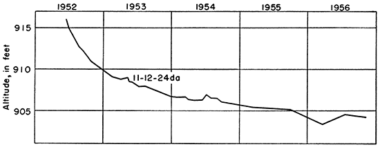
Two observation wells were drilled in Kansas River valley and one in Mill Creek valley during this investigation, and the water levels were measured at intervals from June 1952 through December 1956 (Fig. 5, 6). The rapid water-table decline after the wells were drilled was caused by drought that followed the 1951 Hood; by February 1956 the water table was at least 5 feet below its former level. The rises shown in Figure 6 probably resulted from recharge from precipitation and from bank storage during periods of high water in the river. Discharge from the ground-water reservoir to Mill Creek would be reduced, and water levels in wells on the Hood plain would rise in response to increase in stream level.
Figure 5--Hydrographs of observation well 10-13-19da, 3 miles north of Kansas River, and observation well 10-13-31ba, 1.5 miles north of Kansas River.
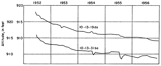
Figure 6--Hydrograph of observation well 11-12-24da, 0.5 mile north of Mill Creek.
Recharge
Recharge is the addition of water to the ground-water reservoir and may be accomplished in several ways. That part of precipitation that does not run off, evaporate, or transpire from plants may percolate down to the water table and recharge the reservoir. Also, if the river level is above the surrounding water table, the river may contribute ground-water recharge. The quantity of precipitation that infiltrates the soil depends upon several factors: the intensity of the rainfall, the slope of the land, the type of soil, the type and amount of vegetation, and the time of the year.
The amount of ground-water recharge in Kansas River valley was not determined in this investigation. Knapp and others (1940, p. 18) estimated that in Soldier Creek basin in eastern Kansas the annual recharge is about half an inch. According to Lohman (1941, p. 45), ground-water recharge from precipitation at Lawrence in Kansas River valley amounts to as much as 10 percent of the precipitation. The normal annual precipitation at Willard is 31.73 inches. On the basis of Lohman's estimate, the average recharge in this area would be about 3 inches, but in drought years there may be no recharge and in wet years the recharge may be much more than 3 inches.
In much of Kansas River valley the surface is fairly Hat and surface runoff is small. Some precipitation accumulates in meander scars and other depressions in the valley, and if these scars are underlain by permeable material, the water soon infiltrates the surface. The scars on the Newman Terrace are underlain by clayey material having low permeability, and water is held in these scars for a long period of time and mostly evaporates.
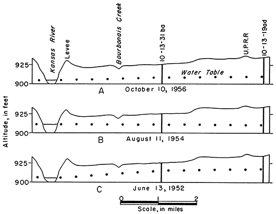
The fact that the water table generally has sloped toward Kansas River during the period of this investigation (Fig. 7A, C), indicates that the river is receiving water from the ground-water reservoir. During high river stages, the slope of the water table near the river is reversed, and the river recharges the alluvium (Fig. 7B). Some of this recharge water from the river is temporary bank storage that soon drains back into the river. When the stage of the river is high, discharge from the ground-water reservoir is decreased or stopped.
Figure 7--Water-table profiles near St. Marys showing the influence of Kansas River stages on recharge and discharge.
Discharge
Ground-water discharge is the removal, by any method, of water from the zone of saturation. Ground water is discharged in Kansas River valley by transpiration and evaporation, by seepage into streams, by subsurface movement into adjacent areas, and by wells.
Transpiration is the process by which water is taken into the root system of plants and discharged into the atmosphere. Alfalfa is probably the only plant in Kansas River valley that has a root system that penetrates to the water table or capillary fringe. Most of the water discharged by transpiration and evaporation is from the soil zone, but some also is discharged from the zone of saturation.
Kansas River receives water by seepage from the ground-water reservoir in most of the valley. Kansas River has been at a low stage during the period of this investigation, permitting considerable quantities of ground-water discharge from the reservoir. Some ground water is discharged by subsurface movement to the east from this section of the valley.
Supplies of domestic, stock, municipal, industrial, and irrigation water in Kansas River valley are derived from wells. The average pumping rate of an irrigation well in this valley is about 700 gpm, and when operating for 24 hours, such a well would remove about 1,000,000 gallons of water from the reservoir. Needed information for computing the total quantity of water pumped annually is not available, but in 1956 the pumpage was small compared to the total discharge. As irrigation increases in Kansas River valley, discharge by irrigation wells may exceed the annual recharge from precipita tion.
Recovery
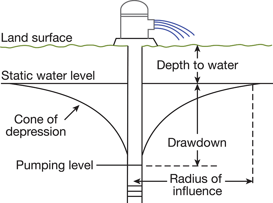
When water is standing in a well, there is equilibrium between the pressure of the water within the well and the pressure of the water outside the well. When water is pumped from a well, the pressure inside the well is reduced, and water moves into the well from the surrounding aquifer. When water is being discharged from the well, the water table in the vicinity of the well is lowered, and a depression is formed somewhat resembling an inverted cone. This depression of the water table is known as "the cone of depression," and the amount that the water level is lowered is called the "drawdown" (Fig. 8).
Figure 8--Diagrammatic section through a well being pumped.
The capacity of a well can be defined as the maximum rate at which it will yield water after the water level during pumping becomes approximately stabilized. The capacity depends on the quantity of water available, the thickness and permeability of the aquifer, and the construction and condition of the well. The capacity of a well generally is expressed in gallons per minute. The specific capacity of a well is its rate of yield per unit of drawdown and is determined by dividing the capacity in gallons per minute by the drawdown in feet. The specific capacity of some of the irrigation wells in Kansas River valley was determined from information obtained from the drillers' tests and is stated under "Remarks" in Table 7.
Utilization
Domestic and stock wells.-About 90 percent of the domestic and stock wells in the valley are driven wells. Many farms have two or more wells, one for domestic supply and the other for stock. The lack of consolidation of the water-bearing material and the shallowness of the water table favor construction of driven wells. The farm wells in the upland are either dug or drilled. Dug wells are walled or curbed with native stone masonry to decrease the possibility of pollution by surface water. Most drilled wells are cased through the unconsolidated material and have a concrete platform at the surface to keep out the surface water.
Irrigation wells
When this investigation started in 1951, no irrigation wells were in use in Kansas River valley between Kiro and Wamego. By the summer of 1954, however, 10 irrigation wells were operating and an old one was being repaired. By July 1956, 52 irrigation wells were in operation. The drought from 1952 through 1956 caused many farmers to irrigate. The estimated yields of irrigation wells range from 500 to 1,500 gpm, and specific capacities range from 40 to 156 gpm per foot of drawdown. Most irrigation wells in Kansas River valley are drilled 30 inches in diameter, have 16- to 18-inch casing, are gravel packed, and penetrate all the water-bearing materials. Most of the irrigation systems are equipped with turbine pumps driven by engines using gasoline, propane, or natural gas for fueL
Industrial wells
Industry is probably the smallest user of ground water in this section of the valley. The alfalfa-dehydrating industry is the only one using ground water, and its process requires very little water.
Public wells
All public water supplies in this area of the valley are obtained from wells in the sand and gravel underlying the Newman Terrace or the Hood plain of Kansas River. The wells are drilled and gravel packed. Wamego, the largest town in the area, pumped an average of 291,600 gallons per day in 1955 from three wells. St. Marys, the next largest town, has four wells approximately 35 feet apart aligned in a northeast-southwest direction. Average daily consumption is about 100,000 gallons. Rossville has two wells that supply 30,000 gallons per day, and Silver Lake has two that supply 35,000 gallons per day.
Aquifer Tests
Three aquifer tests were made in Kansas River valley to determine the ability of the aquifer to transmit water and to yield. water from storage. Procedures for analyzing aquifer test data have been summarized by Brown (1953), and methods of determining permeability have been summarized by Wenzel (1942).
Campbell aquifer test
An aquifer test was made on August 10,1953, using irrigation well 10-10-30ab owned by J. C. Campbell.
The data collected during the test have not been included in this report. An analysis of the data by G. J. Stramel, of the U. S. Geological Survey, is summarized as follows:
The test, in general, was too short to give good results, particularly for the storage coefficient. After analyzing the data by various methods I conclude that the coefficient of transmissibility is about 120,000 gallons per day per foot.
Smith aquifer test
An aquifer test using well 10-11-2ca was made July 9, 1956. The well, an irrigation well owned by Louis Smith, is equipped with a turbine pump powered by a gas engine and is 70.4 feet deep. The alluvium at this site was 86.4 feet thick, and the water level was 27.5 feet below the surface. Three observation wells, IE, 2E, and 3E, about 50 feet deep were installed in a line east of the pumped well at distances of 29, 60, and 90 feet respectively. Well 10-11-2ca was pumped for 21 hours and 15 minutes. The rate of discharge was 550 gpm as estimated from the discharge of gates along the irrigation pipe. Depth to water in the pumped well and observation wells was measured at selected intervals during the pumping period (Table 2).
The coefficient of transmissibility (T) of an aquifer can be determined by plotting the time since pumping started (t) in minutes, divided by the square of the distance to the observation well (r) in feet, on a logarithmic scale and the drawdown (s) in feet on an arithmetic scale, and applying the Theis (1935) nonequilibrium formula as modified by Cooper and Jacob (1946, eq. 8) and restated and adjusted for change in units:
T = (264Q / s) [log10 (t/r2)]
where T is the coefficient of transmissibility, in gpd/ft
Q is the discharge, in gallons per minute,
s is the drawdown of the water level at any distance r from the pumped well, in feet.
Table 2--Water levels measured in pumped well 10-11-2ca and in observation wells 1E, 2E, and 3E during Smith aquifer test, July 9, 1956.
| Time | Time (t) since pumping started, in minutes |
Depth to water, in feet | |||
| Well 10-11-2ca |
1E | 2E | 3E | ||
|---|---|---|---|---|---|
| 12:10 p.m. | Static | 28.10 | |||
| 1:30 | Static | 29.20 | |||
| 2:15 | Static | 29.29 | |||
| 2:16 | Static | 29.43 | |||
| 3:00 | Pump started | ||||
| 3:00:30 | 0.5 | 29.43 | |||
| 3:01 | 1 | 29.95 | |||
| 3:01:30 | 1.5 | 29.27 | 30.22 | ||
| 3:03 | 3 | 30.24 | 29.65 | ||
| 3:04 | 4 | 30.30 | 30.33 | ||
| 3:05 | 5 | 30.32 | 30.35 | ||
| 3:06 | 6 | 30.00 | |||
| 3:07 | 7 | 30.36 | 30.34 | ||
| 3:08 | 8 | 30.35 | |||
| 3:09 | 9 | 30.32 | |||
| 3:10 | 10 | 30.39 | 30.35 | ||
| 3:12 | 12 | 30.35 | |||
| 3:13 | 13 | 31.32 | |||
| 3:15 | 15 | 30.42 | 30.35 | ||
| 3:16 | 16 | 30.33 | |||
| 3:18 | 18 | 31.34 | |||
| 3:20 | 20 | 30.43 | 30.35 | 30.42 | |
| 3:25 | 25 | 30.44 | 30.35 | ||
| 3:26 | 26 | 30.40 | |||
| 3:28 | 28 | 31.26 | |||
| 3:30 | 30 | 30.44 | 30.35 | ||
| 3:31 | 31 | 30.40 | |||
| 3:37 | 37 | 31.40 | |||
| 3:40 | 40 | 30.45 | 30.40 | 30.45 | |
| 3:45 | 45 | 31.46 | |||
| 3:50 | 50 | 30.46 | 30.40 | ||
| 3:51 | 51 | 30.45 | |||
| 3:55 | 55 | 31.47 | |||
| 4:00 | 60 | 30.45 | 30.41 | 30.45 | |
| 4:30 | 90 | 30.49 | 30.42 | 30.45 | |
| 4:32 | 92 | 31.49 | |||
| 5:00 | 120 | 30.50 | 30.44 | 30.46 | |
| 5:02 | 122 | 31.50 | |||
| 5:30 | 150 | 30.50 | 30.45 | 30.46 | |
| 5:32 | 152 | 31.51 | |||
| 6:15 | 195 | 31.53 | 30.51 | 30.46 | 30.50 |
| 7:30 | 270 | 31.57 | 30.53 | 30.48 | 30.55 |
| 9:00 | 360 | 31.59 | 30.55 | 30.50 | 30.57 |
| 12:00 a.m | 540 | 31.61 | 30.59 | 30.54 | 30.60 |
| 4:00 | 780 | 31.65 | 30.60 | 30.55 | 30.61 |
| 8:00 | 1.020 | 31.62 | 30.60 | 30.55 | 30.61 |
| 11:00 | 1.200 | 31.62 | 30.60 | 30.55 | 30.60 |
| 12:15 p.m. | Pump stopped | ||||
Data collected from the observation wells have been plotted on semilogarithmic paper (Fig. 9). The change in water level over one log cycle (δs) in the three observation wells was 0.22. By applying the modified Theis nonequilibrium formula, the coefficient of transmissibility for the test was computed to be 660,000 gpd/ft.
Figure 9--Drawdown in observation wells 1E, 2E, and 3E plotted against log10 t/r2 (time in minutes, divided by square of distance between observation well and pumped well, in feet), Smith aquifer test.
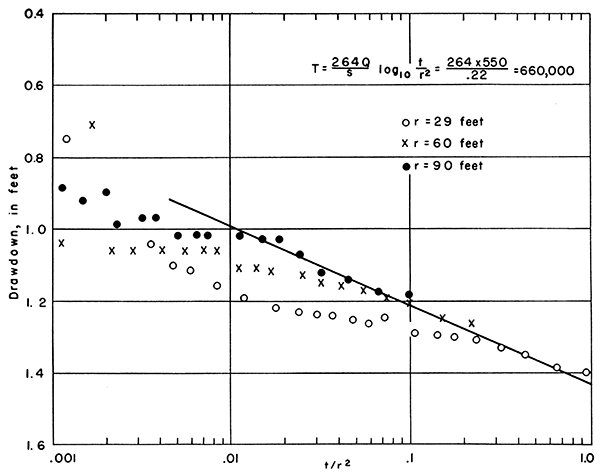
The drawdown in the pumped well at the end of the pumping period was 3.52 feet, and the specific capacity of the well was 156 gallons per foot of drawdown.
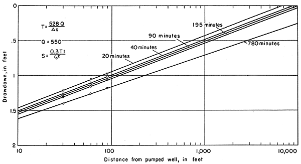
The coefficient of transmissibility (T) of an aquifer can be determined also by use of drawdown data from two or more observation wells. The distance (r) of each observation well from the pumped well is plotted on a logarithmic scale and the drawdown (s) of each observation well on an arithmetic scale. The Thiem formula given by Wenzel (1942) can be reduced to the following formula:
T = (528 Q) / δs
where T is the coefficient of transmissibility, in gpd/ft
Q is the discharge, in gallons per minute,
δs is the drawdown in water level per log cycle of distance of the observation well from the pumped well, in feet.
The drawdown data from observation wells 1E, 2E, and SE were plotted at 20, 40, 90, 195, and 780 minutes (Fig. 10). The values of δs, as determined from Figure 10, and the coefficients of transmissibility are as follows:
| Time since pumping started, minutes |
δs | Coefficient of transmissibility, gpd/ft |
|---|---|---|
| 20 | 0.52 | 558,000 |
| 40 | 0.51 | 569,000 |
| 90 | 0.51 | 569,000 |
| 195 | 0.51 | 569,000 |
| 780 | 0.46 | 631.000 |
Figure 10--Drawdown of water level in observation wells 1E, 2E, and 3E at 20, 40, 90, 195, and 780 minutes plotted against distance from pumped well 10-11-2ca in Smith aquifer test.
Rodgers aquifer test
An aquifer test using well 11-13-3db was made July 26, 1956. The well, an irrigation well owned by Clyde Rodgers, is equipped with a turbine pump powered by electricity, and is 57 feet deep. The well penetrates about 26 feet of saturated material and does not penetrate the total saturated thickness. Two observation wells, 1N and 2N, were installed in a line north of the pumped well at distances of 60 and 90 feet respectively. Well 11-13-3db was pumped for 24 hours at a rate of about 850 gpm as determined from curves of the Berry Irrigation Supply Company. Depth to water was measured in the pumped well and in the observation wells at selected intervals during the pumping period (Table 3).
Table 3--Water levels measured in pumped well 11-13-3db and in observation wells 1N and 2N during Rodgers aquifer test, July 26, 1956.
| Time | Time (t) since pumping started, in minutes |
Depth to water, in feet | ||
| Well 11-13-3db |
1N | 2N | ||
|---|---|---|---|---|
| 6:50 a.m. | Static | 31.73 | ||
| 6:55 | Static | 31.23 | ||
| 6:57 | Static | 31.47 | ||
| 7:00 | Pump started | |||
| 7:00:30 | 0.5 | 35.20 | ||
| 7:01 | 1 | 37.00 | ||
| 7:02 | 2 | 40.10 | ||
| 7:03 | 3 | 40.20 | ||
| 7:05 | 5 | 31.63 | ||
| 7:07 | 7 | 40.20 | ||
| 7:09 | 9 | 40.20 | ||
| 7:10 | 10 | 31.68 | ||
| 7:13 | 13 | 40.25 | ||
| 7:15 | 15 | 40.90 | ||
| 7:18 | 18 | 31.76 | ||
| 7:20 | 20 | 40.59 | ||
| 7:22 | 22 | 31.76 | ||
| 7:23 | 23 | 31.57 | ||
| 7:25 | 25 | 40.35 | ||
| 7:27 | 27 | 31.69 | ||
| 7:28 | 28 | 31.72 | ||
| 7:30 | 30 | 40.05 | ||
| 7:32 | 32 | 31.72 | ||
| 7:33 | 33 | 31.82 | ||
| 7:40 | 40 | 40.38 | ||
| 7:42 | 42 | 31.77 | ||
| 7:45 | 45 | 31.83 | ||
| 7:50 | 50 | 40.64 | ||
| 7:52 | 52 | 31.74 | ||
| 7:54 | 54 | 31.85 | ||
| 8:00 | 60 | 40.65 | ||
| 8:02 | 62 | 31.75 | ||
| 8:03 | 63 | 31.87 | ||
| 8:15 | 75 | 40.65 | ||
| 8:17 | 77 | 31.85 | ||
| 8:18 | 78 | 31.90 | ||
| 8:30 | 90 | 40.39 | ||
| 8:32 | 92 | 31.94 | ||
| 8:33 | 93 | 32.01 | ||
| 8:45 | 105 | 40.02 | ||
| 8:47 | 107 | 31.82 | ||
| 8:48 | 108 | 31.93 | ||
| 9:00 | 120 | 40.02 | ||
| 9:01 | 121 | 31.89 | ||
| 9:02 | 122 | 31.99 | ||
| 9:30 | 150 | 39.93 | ||
| 9:32 | 152 | 32.07 | ||
| 9:34 | 154 | 32.05 | ||
| 10:00 | 180 | 39.90 | ||
| 10:05 | 185 | 32.11 | ||
| 10:06 | 186 | 32.07 | ||
| 11:00 | 240 | 40.20 | ||
| 11:01 | 241 | 32.25 | ||
| 11:02 | 242 | 32.18 | ||
| 12:32 p.m. | 332 | 40.55 | ||
| 12:35 | 335 | 32.40 | ||
| 12:37 | 337 | 32.30 | ||
| 9:00 | 840 | 40.50 | ||
| 9:02 | 842 | 32.80 | ||
| 9:03 | 843 | 32.87 | ||
| 6:52 a.m. | 1.432 | 40.35 | ||
| 6:55 | 1,435 | 33.34 | ||
| 6:57 | 1,437 | 33.27 | ||
| 7:00 | Pump stopped | |||
The rate of discharge of the well varied during the aquifer test, hence the water-level measurements did not plot as a straight line on semilogarithmic paper and no plot of the measurements has been included in this report. Coefficients of transmissibility ranging from 182,000 to 218,000 were determined from a plot of measurements made during the latter part of the test.
The drawdown in the pumped well at the end of the pumping period was 8.6 feet, and the specific capacity of the well was 99 gallons per foot of drawdown.
Quality
The chemical quality of ground water in Kansas River valley is shown by the analyses of 18 samples of water collected from wells (Table 4). The analyses, made in the Water and Sewage Laboratory of the Kansas State Board of Health, show the dissolved mineral content of the water and not the sanitary conditions of the water. The following discussion of the chemical constituents of ground water has been adapted from publications of the U. S. Geological Survey and the State Geological Survey of Kansas.
Table 4--Analysis of water from typical wells in Kansas River valley between Topeka and Wamego Dissolved constituents given in parts per milliona and in equivalents per millionb (in italics).
| Well number |
Depth (feet) |
Geologic source | Date of collection |
Dissolved solids |
Silica (SiO2) |
Iron (Fe) |
Calcium (Ca) |
Magnesium (Mg) |
Sodium and potassium (Na+K) |
Bicarbonate (HCO3) |
Sulfate (SO4) |
Chloride (Cl) |
Fluoride (F) |
Nitrate (NO3) |
Hardness as CaCO3 | ||
|---|---|---|---|---|---|---|---|---|---|---|---|---|---|---|---|---|---|
| Total | Carbonate | Noncarbonate | |||||||||||||||
| 9-16-26db | 50.0 | Newman Terrace deposits | 5-22-1953 | 493 | 14 | 1.0 | 130 6.49 |
29 2.38 |
19 0.83 |
533 8.74 |
17 0.35 |
21 0.59 |
0.1 .01 |
0.97 .02 |
444 | 437 | 7.0 |
| 9-11-33ca | 27 | Newman Terrace deposits | 4-23-1953 | 457 | 23 | 0.05 | 124 6.04 |
16 1.32 |
21 .91 |
433 7.10 |
33 .69 |
15 .42 |
0.1 .01 |
12 .19 |
376 | 365 | 21 |
| 10-10-3cd | 30 | Newman Terrace deposits | 4-22-1953 | 307 | 24 | 0.28 | 62.0 3.09 |
10 .82 |
24 1.04 |
144 2.36 |
64 1.33 |
34 .96 |
0.2 .01 |
18 .29 |
196 | 118 | 78 |
| 10-10-11dc | 31 | Alluvium | 5-22-1953 | 488 | 12 | 0.29 | 131 6.54 |
16 1.32 |
22 .96 |
386 6.33 |
65 1.35 |
24 .68 |
0.3 .02 |
28 .45 |
393 | 316 | 77 |
| 10-10-16ac | 30 | Alluvium | 5-21-1953 | 413 | 14 | 0.14 | 109 5.44 |
14 1.16 |
25 1.09 |
394 6.46 |
38 .79 |
10 .28 |
0.4 .02 |
8.8 .14 |
330 | 323 | 7.0 |
| 10-11-2aa | 29 | Newman Terrace deposits | 4-22-1953 | 481 | 20 | 0.94 | 130 6.49 |
20 1.64 |
15 .65 |
412 6.76 |
78 1.62 |
13 .37 |
0.3 .02 |
1.5 .02 |
406 | 338 | 68 |
| 10-11-5dd | 24 | Alluvium | 4-22-1953 | 496 | 21 | 7.4 | 138 6.89 |
24 1.97 |
14 .61 |
522 8.56 |
32 .67 |
8.0 .23 |
0.2 .01 |
1.3 02 |
443 | 428 | 15 |
| 10-11-15ac | 44 | Buck Creek Terrace deposits | 5-9-1953 | 489 | 3.2 | 0.06 | 105 5.24 |
21 1.73 |
51 2.22 |
429 7.04 |
48 1.00 |
27 .76 |
0.1 .01 |
23 .37 |
348 | 348 | 0.0 |
| 10-12-7aa | 25 | Alluvium | 4-22-1953 | 766 | 23 | 0.65 | 196 9.78 |
25 2.06 |
34 1.48 |
544 8.92 |
77 1.60 |
41 1.16 |
0.2 .01 |
102 1.64 |
592 | 446 | 146 |
| 10-12-16db | 25 | Newman Terrace deposits | 4-22-1953 | 469 | 20 | 1.2 | 116 5.79 |
17 1.40 |
32 1.39 |
410 6.72 |
47 .98 |
24 .68 |
0.3 .02 |
11 .18 |
360 | 336 | 24 |
| 10-12-28cc | 55.7 | Newman Terrace deposits | 5-9-1953 | 552 | 11 | 12.0 | 107 5.34 |
22 1.81 |
73 3.18 |
471 7.72 |
0 0.0 |
86 2.43 |
0.1 .01 |
18 .29 |
358 | 358 | 0.0 |
| 10-13-20cb | 30 | Newman Terrace deposits | 4-28-1953 | 570 | 29 | 0.05 | 148 7.39 |
18 1.48 |
18 .78 |
381 6.25 |
46 .95 |
35 .99 |
0.1 .01 |
88 1.41 |
443 | 312 | 131 |
| 10-13-31bb | 41 | Alluvium | 4-25-1953 | 445 | 19 | 4.9 | 124 6.19 |
15 1.23 |
19 .83 |
418 6.86 |
49 1.02 |
12 .34 |
0.2 .01 |
0.97 .02 |
371 | 343 | 28 |
| 11-13-5dd | 30 | Newman Terrace deposits | 4-28-1953 | 471 | 22 | 0.07 | 128 6.39 |
7.0 .58 |
10 .44 |
229 3.76 |
49 1.02 |
27 .77 |
0.2 .01 |
115 1.85 |
348 | 188 | 160 |
| 11-13-5da | 34.3 | Alluvium | 4-25-1953 | 494 | 20 | 0.05 | 134 6.69 |
15 1.23 |
24 1.04 |
432 7.08 |
46 .95 |
18 .51 |
0.3 .02 |
24 .39 |
396 | 354 | 42 |
| 11-13-20db | 27 | Alluvium | 5-9-1953 | 493 | 24 | 0.33 | 156 7.78 |
14 1.15 |
8.3 .36 |
522 8.56 |
14 .29 |
10 .28 |
0.1 .01 |
9.3 .15 |
446 | 428 | 18 |
| 11-14-21ab | 28 | Alluvium | 4-25-1953 | 917 | 17 | 0.10 | 219 10.93 |
28 2.30 |
33 1.44 |
382 6.26 |
137 2.85 |
65 1.83 |
0.3 .02 |
230 3.70 |
662 | 313 | 349 |
| 11-14-23ab | 28 | Newman Terrace deposits | 4-25-1953 | 397 | 25 | 0.06 | 105 5.24 |
13 1.07 |
19 .83 |
349 5.72 |
44 .92 |
14 .39 |
0.3 .02 |
4.9 .08 |
316 | 286 | 30 |
| a. One part per million is equivalent to one pound of substance per million pounds of water or 8.33 pounds per million gallons of water. b. An equivalent per million is a unit chemical equivalent weight of solute per million unit weights of solution. Concentration in equivalents per million is calculated by dividing the concentration in parts per million by the chemical combining weight of the substance or ion. Factors for converting parts per million of mineral constituents to equivalents per million are given in Table 5. |
|||||||||||||||||
Table 5--Factors for converting parts per million of mineral constituents to equivalents per million.
| Cation | Conversion factor | Anion | Conversion factor |
|---|---|---|---|
| Ca++ | 0.0499 | HCO3- | 0.0164 |
| Mg++ | 0.0822 | SO4-- | 0.0208 |
| Na+ | 0.0435 | Cl- | 0.0282 |
| NO3- | 0.0161 | ||
| F- | 0.0526 |
Dissolved solids
Evaporation of natural water leaves a residue that consists chiefly of mineral matter, and generally of some organic material and a small amount of water of crystallization. Water containing more than 1,000 parts per million of dissolved solids may be used for domestic and irrigation purposes, but it is likely to contain certain constituents in quantities sufficient to make its use unsatisfactory. Water containing less than 500 ppm of dissolved solids generally is suitable for most purposes unless it contains excessive quantities of iron, fluoride, nitrate, or less common constituents that are not discussed subsequently and are not present regularly in well water in eastern Kansas.
The dissolved solids in water derived from alluvium and terrace deposits ranged from 307 to 917 ppm. Water samples from two wells contained more than 600 ppm, and two had less than 400 ppm. Water from wells in the bedrock was not sampled, but Davis and Carlson (1952) reported that water in bedrock wells generally contains more dissolved solids than does the water from alluvium.
Hardness
Hardness of water is generally the property that receives the most attention and is recognized most commonly by its effect when soap is used with the water. Hardness constituents are also the active agents in the formation of the greater part of the scale in steam boilers and in other vessels in which water is heated or evaporated.
In addition to total hardness, the analyses indicate the carbonate hardness and the non carbonate hardness. The carbonate hardness is due to the presence of calcium and magnesium bicarbonate, and it is considerably reduced by boiling. This type of hardness has been called temporary hardness. Noncarbonate hardness is due to sulfates and chlorides of calcium and magnesium and cannot be removed by boiling. This type of hardness has been called permanent hardness. With reference to use with soap, there is no difference between carbonate and noncarbonate hardness. In general, the noncarbonate hardness forms a harder scale in steam boilers than does carbonate hardness.
Water having a hardness of less than 50 ppm generally is regarded as soft, and its treatment for removal of hardness is not necessary under ordinary circumstances. Hardness between 50 and 150 ppm does not interfere seriously with the use of water for most purposes, but it does increase slightly the consumption of soap, and removal of part of the hardness by a softening process is profitable for laundries or other industries using large quantities of soap. Water in the upper part of this range will cause considerable scale in steam boilers. Hardness exceeding 150 ppm is noticeable, and if the hardness is more than 200 ppm, water for household use commonly is softened, or cisterns are installed to collect soft rain water.
In 18 water samples collected for analyses, the total hardness ranged from 196 to 662 ppm. Of the 662 ppm hardness, 349 ppm was noncarbonate hardness. The noncarbonate hardness exceeded 100 ppm in only 3 samples. Water that had the greatest hardness also contained the most dissolved solids.
Iron
Next to hardness, iron is the constituent of water that receives the most attention. The quantity of iron in ground water may differ greatly from place to place even though the water is from the same formation. If water contains more than 0.3 ppm of iron, the iron may precipitate as a reddish sediment. Iron, present in sufficient quantity to give a disagreeable taste and to stain clothing, porcelain ware, and cooking utensils, may be removed from most waters by aeration and filtration, but a few waters require the addition of lime or some other substance.
Iron content of the ground water from alluvium ranged from 0.05 to 12.0 ppm. Three of the 18 samples contained more than 4 ppm and 8 contained more than 0.3 ppm.
Chloride
Water containing less than 150 ppm of chloride is not objectionable for most uses, but water containing more than 500 ppm has an objectionable taste and generally is unsatisfactory for irrigation or industry.
Chloride content of the water samples analyzed ranged from 8 to 86 ppm. In none of the wells inventoried did the water have a salty taste. Insofar as chloride content is concerned, the ground water seems to be satisfactory for domestic and irrigation use.
Fluoride
Although the quantity of fluoride is relatively small compared with other common constituents of water, the amount of fluoride in water that is likely to be used by children should be known. Fluoride in water has been associated with the dental defect known as mottled enamel, which may appear on the teeth of children who, during the formation of their permanent teeth, habitually drink water containing excessive fluoride. Water containing more than 1.5 ppm of fluoride is likely to produce mottled enamel, If the water contains as much as 4 ppm of fluoride, 90 percent of the children exposed are likely to have mottled tooth enamel, and 35 percent or more of the cases will be classed as moderate or worse (Dean, 1936). Small quantities of fluoride, not sufficient to cause mottled enamel, prove beneficial by decreasing tooth decay. Fluoride content of water from the alluvium of Kansas River valley ranged from 0.1 to 0.4 ppm and averaged about 0.3 ppm.
Nitrate
The nitrate content of water from wells in the area ranged from 0.97 to 230 ppm. Three of the 18 samples contained more than 90 ppm of nitrate; the rest had less than 30 ppm. The difference in nitrate content of the water is considerable, but seemingly is not related to any geologic condition.
A large amount of nitrate in water may cause cyanosis when the water is used in preparation of a baby's formula. Water that contains more than 90 ppm of nitrate is regarded by the Kansas State Board of Health as likely to cause infant cyanosis, whereas water containing less than 45 ppm generally is considered safe.
Water for Irrigation
This discussion of suitability of water for irrigation is adapted from Agriculture Handbook No. 60 of the U. S. Department of Agriculture.
Successful irrigation depends not only upon the supplying of irrigation water to the land but also the control of the salinity and alkalinity of the soiL Quality of irrigation water, irrigation practices, and drainage are involved in salinity and alkalinity control. Soil that was originally nonsaline and non alkali may become unproductive if excessive soluble salts or exchangeable sodium are allowed to accumulate because of improper irrigation and soil-management practices or inadequate drainage.
In areas of sufficient rainfall and ideal soil conditions the soluble salts originally present in the soil or added to the soil by water are carried downward by the water and ultimately reach the water table. This process of dissolving and transporting soluble salts by the downward movement of water through the soil is called leaching. If the amount of water applied to the soil is not in excess of the amount needed by plants, there will be no downward percolation of water below the root zone, and mineral matter will accumulate. Likewise, impermeable soil zones near the surface can retard the downward movement of water, resulting in water-logging of the soil and deposition of salts. Leaching requires the free passage of water through and away from the root zone, hence, unless drainage is adequate, attempts at leaching may not be successful.
The characteristics of an irrigation water that seem to be most important in determining its quality are: (1) total concentration of soluble salts; (2) relative proportion of sodium to other cations (magnesium, calcium, and potassium); (3) concentration of boron or other elements that may be toxic; and ( 4) under some conditions, the bicarbonate concentration as related to the concentration of calcium plus magnesium.
For purposes of diagnosis and classification of irrigation water, the total concentration of soluble salts can be adequately expressed in terms of electrical conductivity, which is a measure of the ability of the inorganic salts in solution to conduct an electrical current, and which in soils work usually is expressed in terms of micromhos per centimeter. The electrical conductivity can be determined in the laboratory, or an approximation of the electrical conductivity may be obtained by multiplying the total equivalents per million (Table 5) of calcium, sodium, magnesium, and potassium by 100, or by dividing the total dissolved solids in parts per million by 0.64.
In general, waters having electrical conductivity values below 750 micromhos are satisfactory for irrigation insofar as salt content is concerned, although salt-sensitive crops such as strawberries, green beans, and red clover may be affected adversely by irrigation water having an electrical conductivity value in the range of 250 to 750 micromhos. Waters in the range of 750 to 2,250 micromhos are widely used, and satisfactory crop growth is obtained under good management and favorable drainage, but saline conditions will develop if leaching and drainage are inadequate. Use of waters having conductivity values above 2,250 micromhos is the exception, and very few projects can be cited where such waters have been used successfully.
In the past the relative proportion of sodium to other cations in irrigation water usually has been expressed simply as percent sodium. According to the U. S. Department of Agriculture, however, the sodium-adsorption ratio (SAR), used to express the relative activity of sodium ions in exchange reactions with soil, is a much better measure of the suitability of water for irrigation. The sodium-adsorption ratio may be determined by use of the nomogram shown in Figure 11. In using the nomogram to determine the sodium-adsorption ratio of a water, the concentration of sodium expressed in equivalents per million (Table 5) is plotted on the left-hand scale (A), and the concentration of calcium plus magnesium expressed in equivalents per million is plotted on the right-hand scale (B). The point where the line connecting these two points intersects the sodium-adsorption-ratio scale (C) is the sodium-adsorption ratio of the water. When the sodium-adsorption ratio and the electrical conductivity of a water are known, the suitability of the water for irrigation can be determined by plotting these values on the diagram shown in Figure 12. Low-sodium water (S1) can be used for irrigation on almost all soils with little danger of the development of harmful levels of exchangeable sodium. Medium-sodium water (S2) will present an appreciable sodium hazard in certain fine-textured soils, especially under low-leaching conditions. This water may be safely used on coarse-textured or organic soils having good permeability. High-sodium water (S3) may produce harmful levels of exchangeable sodium in most soils and will require special soil management, such as good drainage, high leaching, and additions of organic matter. Very high sodium water (S4) is generally unsatisfactory for irrigation unless special action is taken, such as addition of gypsum to the soil.
Figure 11--Nomogram for determining value of sodium-adsorption ratio of irrigation water.
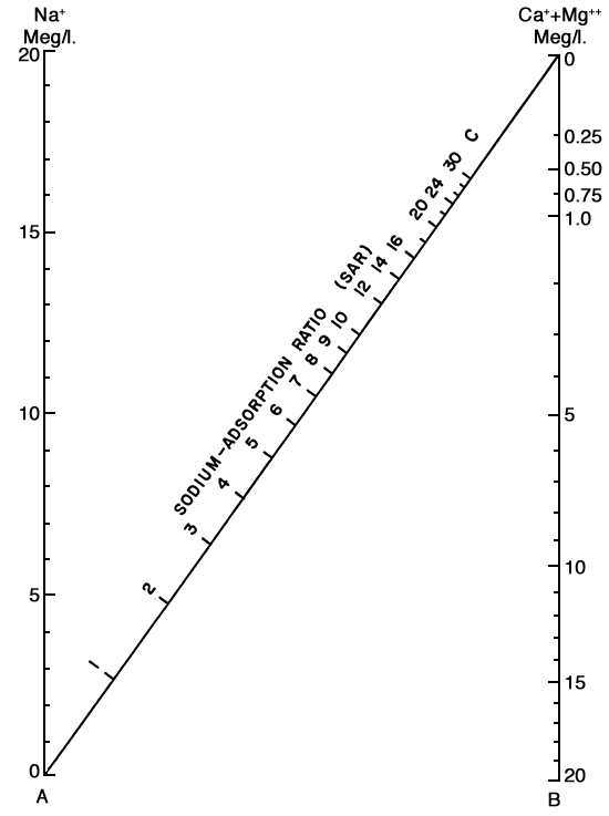
Figure 12--Diagram showing classification of water for irrigation.
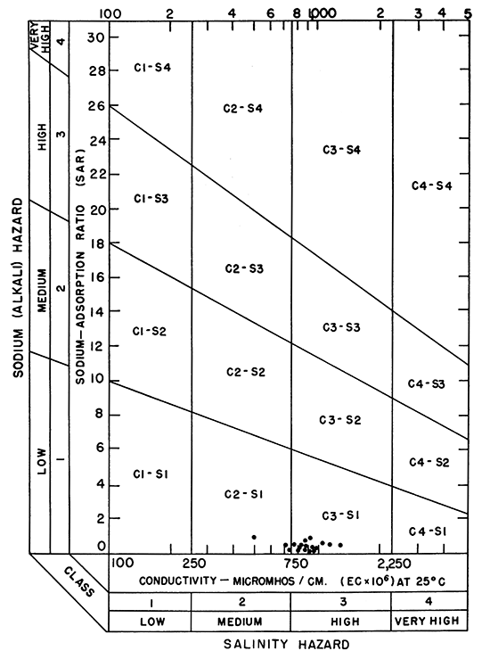
Low-salinity water (C1) can be used for irrigation of most crops on most soils with little likelihood that soil salinity will develop. Medium-salinity water (C2) can be used if a moderate amount of leaching occurs. Crops with moderate salt tolerances, such as potatoes, corn, wheat, oats, and alfalfa, can be irrigated with C2 water without special practices. High-salinity water (C3) cannot be used on soils with restricted drainage. Very high salinity water (C4) can be used only on certain crops and then only when special practices are followed.
Boron is essential to normal plant growth, but the quantity required is very small. Crops differ greatly in their boron tolerances, but in general, the ordinary field crops common to Kansas are not adversely affected by boron concentrations of less than 1 ppm.
Table 6--The sodium-adsorption ratio (SAR), conductivity, and class of water samples shown on Figure 12. (Chemical analyses of water samples are given in Table 4).
| Well number | SAR | Electrical conductivity, micromhos |
Class |
|---|---|---|---|
| 9-10-26db | 0.40 | 970 | C3-S1 |
| 9-11-33ca | 0.50 | 830 | C3-S1 |
| 10-10-3cd | 0.76 | 500 | C2-S1 |
| 10-10-11dc | 0.46 | 880 | C3-S1 |
| 10-10-16ac | 0.64 | 770 | C3-S1 |
| 10-11-2aa | 0.32 | 880 | C3-S1 |
| 10-11-5dd | 0.30 | 950 | C3-S1 |
| 10-11-15ac | l.20 | 920 | C3-S1 |
| 10-12-7aa | 0.60 | 1,330 | C3-S1 |
| 10-12-16db | 0.80 | 860 | C3-S1 |
| 10-12-28cc | 0.75 | 1,030 | C3-S1 |
| 10-13-20cb | 0.32 | 960 | C3-S1 |
| 10-13-31bb | 0.40 | 820 | C3-S1 |
| 11-13-5da | 0.52 | 800 | C3-S1 |
| 11-13-12db | 0.24 | 740 | C2-S1 |
| 11-14-20db | 0.12 | 930 | C3-S1 |
| 11-14-21ab | 0.60 | 1,470 | C3-S1 |
| 11-14-23ab | 0.52 | 710 | C2-S1 |
The boron content of water samples from Kansas River valley was not determined, but other investigations in the general area have not found excessive concentration of boron in the water.
Of the waters sampled in Kansas River valley, none was unsuitable for irrigation (Fig. 12). None of the samples had a sodium-adsorption ratio greater than 1.2, and for most of the samples it was below 0.75 (Table 6). The electrical conductivity ranged from 500 to 1,470 micromhos and for most samples was between 750 and 1,000. Most soils in Kansas River valley drain adequately, hence waters having conductivities of this magnitude are not detrimental.
Prev Page--Geomorphology || Next Page--Well Records
Kansas Geological Survey, Geology
Placed on web June 16, 2014; originally published March 1959.
Comments to webadmin@kgs.ku.edu
The URL for this page is http://www.kgs.ku.edu/Publications/Bulletins/135/06_water.html