Kansas Geological Survey, Petrophysical Series 3
1Schlumberger Well Services
3Kansas Geological Survey
3Marathon Oil Company
[Originally published in 1982 as Kansas Geological Survey Petrophysical Series 3. This is, in general, the original text as published. The information has not been updated. An Acrobat PDF file containing the complete report is available (3.8 MB). Plate 1 is in a separate file, linked below.]
Core and cuttings studies of the Viola Limestone (Middle to Upper Ordovician) in south-central Kansas were integrated with numerical analyses of wireline logs in a composite evaluation of lithofacies variation. Two basic end-member facies were recognized; a low-porosity limestone of crinoidal packstones and grainstones, and a moderately porous cherty dolomitic limestone representing dolomitized wackestones and mudstones. These facies can be traced from both cuttings profiles and wireline log traces across the area as correlative subdivisions of the Viola. Fourier analysis of fine-scale variation of log-derived mineralogy suggests that facies migration was cyclic rather than episodic, in response to either an eustatic or tectonic control.
Lateral changes in facies, as interpreted from core cuttings, show a basic parallelism with the Central Kansas Arch. These range outwards from a somewhat restricted facies of sparsely fossiliferous wackestones and mudstones to crinoid packstones and grainstones representative of higher energy, open-marine environments. The influence of the Pratt Anticline as a positive feature contemporaneous with deposition is suggested in the upper Viola from core evidence and in the lower Viola from log analysis. In both instances, these appear as a relative enhancement of a calcite mud component on the structural axis, which graded outwards to less micritic higher energy facies on the flanks.
Computer processing of neutron, sonic, and density logs resulted in an interpretative lithofacies map in which the patterns reflect a complex history of deposition, diagenesis, and erosion. The disposition of limestone and dolomite facies as the dominant aspect of the Viola was dictated by erosional bevelling of the formation in Devonian and early Pennsylvanian times. On a regional scale, the Viola thins to the east with marked local variation controlled by differential fault-block movement. The lithofacies may also outline a region which represents solution weathering of the Viola to produce karstic carbonate zones and extensive deposits of residual chert. The map shows a distinctive grain which coincides with southerly continuations of fault trends associated with the Precambrian Central North American Rift System. These faults appear to have been intermittently active throughout the Paleozoic, influencing depositional trends, diagenetic patterns, erosional history, and the location of traps for Viola oil fields.
Plate 1--Lithofacies and structural map of the Viola Limestone in south-central Kansas computed from Neutron, Sonic, and Density logs
Wireline logs have been applied routinely for decades in the correlation of distinctive marker horizons and the boundaries of major lithologic units In the subsurface. In regional studies, log picks of stratigraphic markers and their vertical separations are used to map out surfaces of structural elevation and areal changes in thickness. These are important aids in both the understanding of the geological history of a basin and the search for mineral resources. However, this information alone is restrictive, since it merely describes the variations in shape and size of subsurface formations.
Qualitative interpretations of the character of log curves gives useful indications of lithology, but detailed lithofacies studies have drawn heavily on cuttings and core descriptions. Both of these traditional sources of data have practical limitations to their application in regional studies. Cores provide the most comprehensive information, but are generally severely restricted in both areal coverage and vertical sampling because of the expense of core recovery operations. Cuttings provide the most common source of lithologic information but are dogged by a variety of problems. Skillful work is required to identify contamination by caved materials and the effect of selective bias in description by different geologists. Allowance must be made for errors caused by the lag times of the cuttings' journey to the surface and by the differential flotation of components within the mud column. Estimation procedures are, at best, semiquantitative and often distorted by the selective comminution of more friable components by the drill-bit.
Relatively recent advances in log analysis and their trial in field studies have introduced alternative methods in the analysis of lithofacies which show great potential in augmenting cuttings and core information. Many years ago log analysis was as much an art as a science when used in the search for oil and gas reservoir horizons. The integration of simple theoretical physics with laboratory experiments laid the groundwork for mathematically interrelating log measurements and reservoir properties. The equations have proved their worth in providing reasonable quantitative estimates of porosities and hydrocarbon saturations from wireline logs. However, recognition of the complexity of subsurface geology has encouraged more sophisticated extensions of earlier methods to accommodate the variation in mineral composition of potential reservoir horizons. Although the fundamental aim of the log analyst is the enhancement of estimations of pore properties, the by-product of this effort has been the development of new methods for lithofacies analysis.
In a literal sense, wireline logs are remotely sensed data from the subsurface, recording the physical properties of rocks. These measurements are made by electrical, nuclear, and acoustic devices and some may seem to be alien to "real geology." However, the agonizingly time-consuming wet chemical procedures of conventional rock analysis largely have been replaced by X-ray diffraction and fluorescence, neutron activation, and other nuclear methods. The fundamental differences between modern geochemical laboratory practice and logging operations now lie in the problems introduced by telemetry, sample size resolution, and the less than ideal environment of the typical borehole.
A particular advantage of wireline logs is their intrinsic numerical character which makes them amenable to bulk processing by computer. As a result, quantitative transformations of log readings to stratigraphic profiles of individual wells or to lithofacies maps of entire areas are now a practical possibility. However, just as satellite image analysis requires a certain element of "ground truth" as a necessary ingredient for intelligent work, subsurface rock samples are the appropriate guides for log analyses. In a detailed study, core and cuttings serve two crucial functions: validation and interpretation. Log analysis of lithofacies must first be consistent with the geology of the formation found by the drill-bit. At another level, the less tangible rock characteristics of paleontology, sedimentology, and diagenesis are the necessary keys for providing genetic meanings to patterns derived from logs.
The notion of integrating logs with cuttings and core samples in a regional stratigraphic study is not a new one. However, this report describes a change in emphasis with the central role being played by log analysis while core and cuttings provide a supporting function. Since many of the mathematical techniques described are relatively new, the study is in part an experiment to determine the practicality of computer methods in regional examinations of lithofacies analysis based on logs. The results are interpreted in terms of depositional facies, diagenetic processes, and structural history, which have both academic interest and practical implications.
The target formation of this report is the Viola Limestone (Middle to Upper Ordovician) and the study area is located in a four-county region of south-central Kansas (Fig. 1). This section and area were selected to satisfy several criteria:
Figure 1--Location of study area in Kansas.
Throughout the Ordovician, paleogeography and sedimentation of the cratonic areas of the Midcontinent region were controlled primarily by the Transcontinental Arch, and by the position of the North American plate with respect to the Earth's latitudinal belts (Ross, 1976). Evidence of Late Ordovician glaciation (Sheehan, 1973) as well as latitudinal biotope variations (Berry and Boucot, 1970) support the hypothesis that extensive polar ice caps created a more pronounced climatic zonation than that postulated for the Cambrian and Late Silurian (Spjeldnaen, 1976). The Transcontinental Arch represented a nearly continuous land bridge in the Early Ordovician, but became inundated over wide areas at the close of the period. Its known extension covered an area from New Mexico to Minnesota across the Midcontinent.
The Viola Limestone in south-central Kansas was deposited in an extensive epicontinental sea that covered a large part of North America during Middle to Late Ordovician time (Witzke, 1980). Shaw (1964) and Irwin (1965) both proposed facies patterns for deposition in epicontinental seas with low sea-floor slopes. They postulated that environments would develop as broad adjacent bands parallel to the paleoshoreline. The widths of the bands are dependent on the slope of the sea floor, with narrower bands developing in areas of greater slope.
The widespread distribution of facies in the Viola implies deposition in extensive belts, though not on the scale of hundreds of miles as proposed by Irwin (1965) for deposition on sea floors with slopes of less than 1 foot per mile. There is, however, no known shoreline present in the area during Viola time, although there was a submerged arch trending northwest from the Chautauqua Arch towards the Central Kansas Uplift (Adkison, 1972). This arch will be referred to as the Central Kansas Arch following Rich (1933), and includes the pre-Mississippian elements of the Chautauqua and the Ellis arches (Fig. 2). The Ellis Arch is the pre-Mississippian structure which was ancestral to the Central Kansas Uplift (Jewett, 1951). The general depositional setting was an open-marine environment shallowing towards this arch, with semirestricted and very restricted environments developed where water depths decreased with concomitant decreases in circulation and probable increase in salinity.
Figure 2--Major pre-Mississippian structural features of Kansas.
The Viola Limestone of south-central Kansas consists of limestones, dolomites, and cherts. Although several geologists such as Taylor (1947) and Ver Wiebe (1948) subdivided the Viola into informal lithologic units, Lee (1956) concluded that the Viola could not be zoned on a regional basis. Adkison (1972) made a detailed study of the structure and stratigraphy of the Viola across the Sedgwick Basin and was able to trace some individual units across limited areas. However, his lithofacies map of the area of this report shows only a simple subdivision between zones of residual chert development and zones with no residual chert. He made a tentative interpretation of karst topography and possible evidence of cavern fillings in some wells to explain thickness variations of the Viola. Adkison mapped a triangular area extending southward from the southern flank of the central Kansas Uplift into Pratt County in which the Viola was either partly or entirely residual chert. This chert appears to be the residue of extensive solution weathering of cherty Viola carbonates in Late Devonian, Late Mississippian, and Early Pennsylvanian times.
St. Clair (1981) made detailed examinations of slabbed Viola core and thin-sections from ten wells in Barber and Pratt counties. Locations of these cores are shown in Figure 3 and listed in Table 1. The limited coverage restricted detailed analysis to the eastern half of the total study area (unshaded region of Fig. 3). The purpose of this study was to identify depositional facies, summarize their compositions, trace lateral variations, and reconstruct diagenetic histories. Sample logs on file at the Kansas Geological Survey were used to determine the distribution of facies in areas where no core was available.
Figure 3--Map showing location of cores (stars) used in this study. Interpretations from core data were restricted to the unshaded portion of the total study area. Core numbers correspond to numbers in Table 1.
Table 1--Cores used in this study.
| Company Well |
County | Section Township Range |
Section location |
Depth, meters (feet) |
|
|---|---|---|---|---|---|
| 1 | Sinclair-Prairie 1 Degeer |
Barber | 34 32S 15W | NE NW NE | 1508-1551 (4948-5087) |
| 2 | Sinclair 1 Alice Gentry |
Barber | 1 33S 15W | NE C NE | 1571-1594 (5106-5231) |
| 3 | Sinclair-Prairie 1 M. Binning |
Barber | 26 32S 13W | SE SE SW | 1454-1481 (4769-4860) |
| 4 | Lario 2 Randles |
Barber | 34 32S 12W | C NE NE | 1417-1447 (4649-4746) |
| 5 | I.T.I.O. 1 George |
Barber | 12 33S 1OW | C SE SW | 1433-1458 (4702-4782) |
| 6 | Carter 1 Lytle |
Barber | 6 32S 14W | C NE NW | 1435-1473 (4709-4832) |
| 7 | Sinclair-Prairie 1 A. Oldfather |
Barber | 18 31S 14W | NE NE SW | 1349-1389 (4426-4556) |
| 8 | Sinclair 4 G. Oldfather |
Barber | 7 31S 14W | SW NW SE | 1319-1357 (4328-4453) |
| 9 | Bridgeport 1-1 Brown |
Pratt | 25 29S 13W | SE SE SW | 1361-1400 (4465-4592) |
| 3 | Sinclair-Prairie 1 Blurton |
Pratt | 22 28S 12W | NE SE NW | 1309-1343 (4294-4407) |
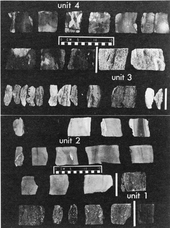
As a result of her study, St. Clair was able to subdivide the Viola in the eastern half of the study area into four mappable units, which were informally named the basal limestone, the lower cherty dolomitic limestone, the upper limestone and the upper cherty dolomitic limestone. The petrographic characteristics and fossil content of these units are summarized graphically as a composite section in Figure 4. Photographs of all four facies units from a slabbed core in a single well (Degeer #1, 34-32S-1 5W, Barber County) are shown in Figure 5.
Figure 4--Generalized stratigraphic section of the Viola Limestone in south-central Kansas.
Figure 5--Slabbed core of Viola Limestone from Degeer #1 (34-32S-15W). Basal limestone = 1; lower cherty dolomitic limestone = 2; upper limestone = 3; upper cherty dolomitic limestone = 4. Stratigraphic depth increases from top to bottom and from left to right.
The basal limestone forms an almost continuous sheet across the study area and has a characteristic "tight-lime" (low porosity) log response that is useful for locating the boundary between the Viola and the underlying Simpson Group. The unit ranges in thickness from 5 to 25 feet and can be characterized as a crinoid packstone-grainstone facies limestone (Figs. 6 and 7). Fossil fragments other than crinoids include brachiopods, bryozoans, and trilobites, with occasional molluscs, ostracodes, sponge spicules, and unidentified phosphatic f os s !is. Pellets and intraclasts are rare. The interparticle areas are largely filled with optically continuous calcite overgrowths on the crinoids, with minor amounts of bladed cement on the other fossil fragments. Lime mud is present, but only rarely does it occur in large enough quantities to prevent extensive cementation by syntaxial overgrowths on the crinoids. The fossil fragments have sufficient grain contacts to form a supporting framework. In some cases, pressure solution has resulted in embayed and sutured grain contacts.
Figure 6--Slabbed core of crinoid packstone-grainstone facies of the basal and upper limestones.
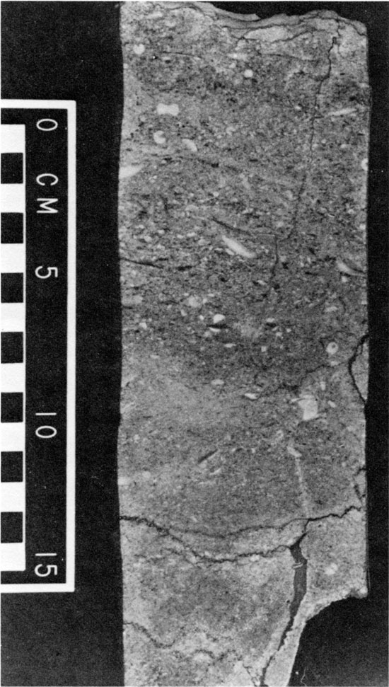
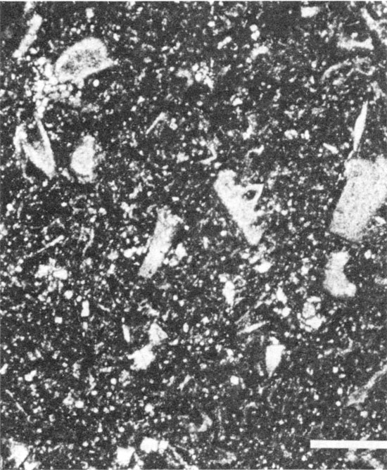
Figure 7--Photomicrograph of crinoid packstone-grainstone facies of the basal and upper limestones. Note the abundant syntaxial cement on the crinoids, the micritic rims on the trilobites, and the dolomite rhombs in the bryozoans. The bar scale is 1 mm.
The fossils vary in their state of preservation. The crinoids, which are the best preserved, may be partially replaced by dolomite or silica and occasionally display peripheral micritization due to algal or fungi borings (Bathurst, 1966). Generally, the trilobites are slightly abraded and show the most extensive peripheral micritization. Brachiopods usually are highly fragmented and abraded and most commonly are silicified, while bryozoans show the least preservation and often are completely recrystallized or dolomitized.
Adkison (1972) reported cross-bedding in the basal limestone, but none was recognized in samples in this study. Green shale stringers occur in places, as do lenses of fine-grained dolomite. These lenses may be up to 1 cm (0.39 inch) thick and probably were originally lime mud. Large intraclasts, up to 2.5 cm (1 inch) long, which were ripped up from these lenses, also occur.
In addition to dolomitized mud lenses, dolomite also occurs as well-developed rhombs ranging in size from 0.08 to 0.26 mm (0.003 to 0.01 inch). These are found replacing inter- and intraparticle lime mud and also may replace fossils. The amount of dolomite increases as the amount of original lime mud increases. This probably is due to the greater ease of dolomitization of original aragonitic or high-magnesium calcite mud (Cloud, 1962). Also, since the lime mud impedes the complete filling of interparticle areas by syntaxial overgrowths, rocks with greater amounts of lime mud may have been more porous than those with little mud, also aiding the process of dolomitization.
Chert nodules are rare in this facies. Where they do occur, they are composed of a mixture of cryptocrystal line and microcrystal line quartz and chalcedony with abundant calcite inclusions. Long axes of the nodules may be up to 5 cm (2.0 inches) in length and are roughly oriented parallel to bedding. The nodules contain numerous fossil ghosts of trilobites, brachiopods, bryozoans, crinoids, and ostracodes and have a mottled light brown, gray, and white coloration. The contact between nodules and the carbonate matrix is abrupt. Chert nodules are found in those samples having the highest content of original lime mud and which have consequently been dolomitized most extensively.
This unit originally was present throughout the study area, but has since been removed by erosion over the Pratt Anticline. The unit ranges in thickness from 10 to 104 feet and consists of dolomitized mixed-skeletal wackestones and dolomitized mudstones.
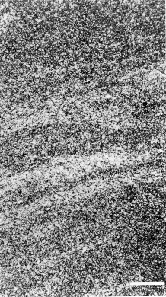
The lower part consists of green to light-brown or gray, argillaceous, cherty dolomite mudstones, which commonly are laminated or mottled (Figs. 8 and 9). The dolomite is very fine to medium grained and occurs as rhombs or subhedral crystals. Many crystals are multiply zoned with concentric outlines of alternating ferroan and nonferroan dolomite. Ferroan saddle dolomite that has a warped crystal lattice (Radke and Mathis, 1979) occurs as a cement which partially fills the remaining voids.
Figure 8--Slabbed core of laminated dolomitic mudstone facies in the lower cherty dolomitic limestone. Note the burrows, indicated by arrows.
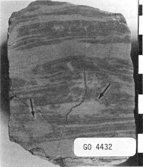
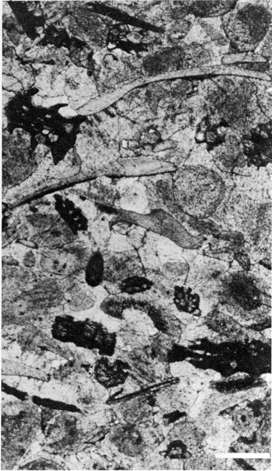
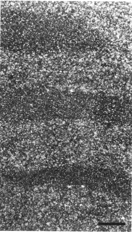
Figure 9--Photomicrograph of laminated dolomitic mudstone facies in the lower cherty dolomitic limestone. The bar scale is 1 mm.
Fossils of crinoids, brachiopods, trilobites, bryozoans, and ostracodes are rarely present. Most of the crinoids are replaced by large single crystals of dolomite. Other fossils are associated with chert nodules and are either partially or totally silicified, depending upon completeness of chert-nodule formation.
Laminations occur as alternating layers of medium- and fine-grained crystals, which may reflect original sediment size differences. Burrows are common and may be filled by dolomite rhombs of a different size than those in the undisturbed sediment. Aside from these features, the size distribution of dolomite crystals is uniform, implying recrystallization from a sediment of uniform grain size, such as lime mud.
Chert nodules are white or gray with white borders, may exceed 8.5 cm (3 inches) in length, and are composed of cryptocrystal line quartz. Some chert nodules display ghosts of fossils that are not present in the dolomitized matrix. This may be interpreted as either preservation of the original texture and composition of the sediment in the chert nodule, or as preferential silicification around fossils. The uniform texture of the dolomite and the occurrence of partial silicification in the vicinity of fossils supports the latter hypothesis. The fossils may have been washed in and created a local micro-environment favorable to silicification.
A pale-green or light-gray, argillaceous, cherty, dolomitic, mixed-skeletal wackestone occurs at the top of this unit (Figs. 10 and 11). By analogy with modern shallow-water carbonates we can infer that the matrix probably was originally aragonitic and high-magnesium calcite mud, and has since been partially or completely dolomitized (Cloud, 1962). The dolomite exists as well-formed rhombs ranging in size from 0.08 to 0.26 mm (0.003 to 0.01 inch), and as very fine-grained anhedral crystals. The dolomite rhombs may exhibit as many as five different stages of growth in the form of alternating layers of nonferroan and ferroan dolomite or as dust rings that formed on the surface of the crystals between growth stages. Fine-grained neomorphic calcite spar may exist between the dolomite rhombs. According to Mossler (1971), this indicates that early dolomitization probably preceded alteration of the matrix to low-magnesium calcite.
Figure 10--Slabbed core of dolomitic mixed-skeletal wackestone facies at the top of the lower cherty dolomitic limestone.
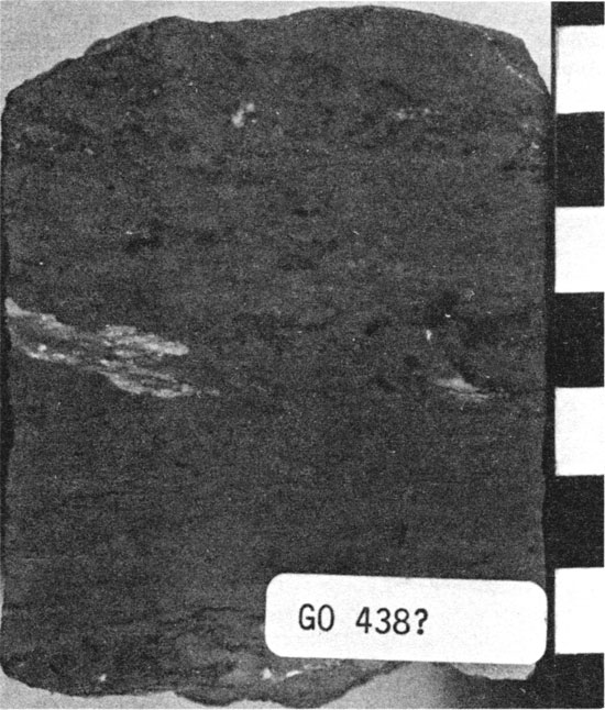
Figure 11--Photomicrograph of dolomitic mixed-skeletal wackestone facies at the top of the lower cherty dolomitic limestone. Note the completely dolomitized matrix, the lack of syntaxial rims on the crinoids, and the partial silicification of the brachiopod fragment (arrow). The bar scale is 1 mm.
Fossils in this facies include crinoids, bryozoans, brachiopods, trilobites, phosphatic brachiopods, sponge spicules, ostracodes, and unidentified phosphatic skeletal fragments. Only a few of these are present in a single sample. Other constituents include phosphatic pellets and peloids which probably are recrystallized skeletal fragments. Fossils which were originally calcite generally are still calcite, but they may be partially silicified to chalcedony or microcrystalline quartz. Brachiopods and crinoids are most commonly silicified. Some fossils, usually crinoids, are dolomitized and may be replaced by a single crystal of dolomite or by many tiny rhombs. Bryozoans whose zooecia have been filled with mud also tend to be partially replaced by dolomite.
The chert nodules in the mixed skeletal wackestone may be up to 5.2 cm (2.04 inches) long. They are light gray or white and are composed of crypto crystal line quartz. Usually, the contact between the nodules and the carbonate matrix is sharp.
The upper limestone is present only in the southwestern half of the study area, having been removed by erosion in the northeast. The unit ranges in thickness from 4 to 32 feet and consists of crinoid packstones and grainstones. In almost all respects, the petrographic characteristics of the upper limestone are similar to those of the basal limestone.
This unit occurs only in the western and southern part of the area, having been removed by erosion to the east and the north. It ranges in thickness from 4 to 48 feet and consists of mixed-skeletal wackestones, with some dolomitic intraclast wackestones and dolomitic mudstones over the Pratt Anticline.
Pale-green or light-gray, mixed-skeletal wackestones (Figs. 12 and 13) were deposited in the southern part of the study area. The matrix of these rocks probably was originally aragonitic and high-magnesium calcite mud, which has since been either completely replaced by dolomite or recrystallized to neomorphic calcite spar with minor replacement dolomite.
Figure 12--Slabbed core of mixed-skeletal wackestone facies of the upper cherty dolomitic limestone.
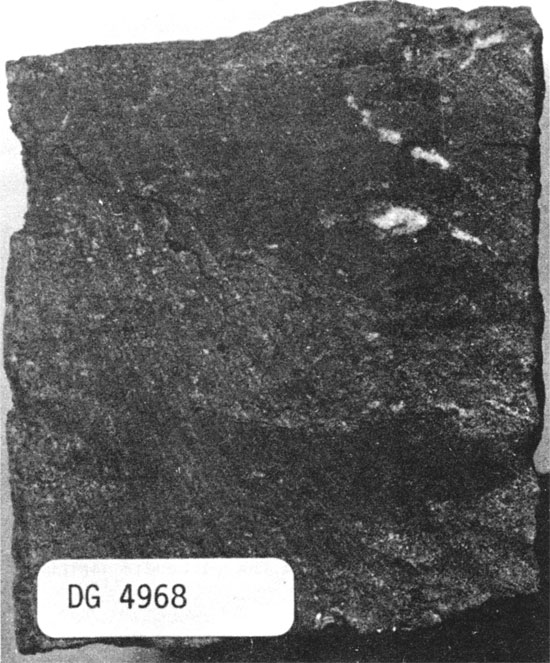
Figure 13--Photomicrograph of mixed-skeletal wackestone facies of the upper cherty dolomitic limestone. Note that the matrix has been partially dolomitized. The bar scale is 1 mm.
The dolomite matrix consists of micritic to very fine-grained anhedral crystals and fine-grained clear rhombic crystals. Ferroan dolomite occurs only as a very coarse-grained, void-filling, saddle dolomite cement.
Where the matrix is neomorphic calcite spar, it may consist entirely of extremely fine-grained crystals, or it may be fine- to medium-grained, subhedral crystals. In some places the matrix has a texture similar to that of the dolomite matrix of the lower cherty dolomitic limestone, with extremely fine-grained anhedral crystals mixed with very fine- to fine-grained calcite rhombs. In places, clear, fine-grained, rhombic dolomite occurs in these samples.
Fossils in these mixed-skeletal wackestones include crinoids, brachiopods, trilobites, bryozoans, ostracodes, mollusks, and sponge spicules. Other constituents include peloids, which probably are fossils that have been micritized beyond recognition, and phosphatic pellets. Generally, no more than three fossil constituents are present at any given location, and usually there are only one or two varieties of fossils. Crinoids are the most common, followed by trilobites and ostracodes. Syntaxial overgrowths on the crinoids, where present, are poorly developed. The fossils usually are calcite but may be partially or completely replaced by cryptocrystal line quartz. Crinoids also are commonly replaced by single crystals of dolomite.
In general, the degree of dolomitization of the original matrix increases as the number of fossils decreases. This may imply that the depositional environment became more restricted, possibly by a sharp increase or decrease in salinity that promoted penecontemporaneous dolomitization.
Chert nodules in the skeletal wackestones are white or gray with white borders, are composed of cryptocrystal line quartz, and exceed 6.5 cm (2.55 inches) in length. Where the formation of nodules is complete, nodules have abrupt contacts with the carbonate matrix. In some samples, incomplete formation of chert nodules is indicated by curved bands of cryptocrystal line quartz, with the most intensive silicification occurring at the outer edges of the bands. If the silica replaced a calcite matrix, the calcite crystals often are rimmed with micritic dolomite. The amount of dolomite increases toward the center of the nodule. Quartz also occurs as a drusy, void-filling cement, which is fine- to very fine-grained with crystal size increasing away from the edge of the void.
North of the area of occurrence of mixed-skeletal wackestones, along the edge of the Pratt Anticline, this unit consists of dolomitized intraclast wackestones (Figs. 14 and 15) and laminated dolomitized mudstones. These rocks are green and gray or pale green and white.
Figure 14--Slabbed core of dolomitic intraclast wackestone facies of the upper cherty dolomitic limestone. Arrows point to the intraclasts.
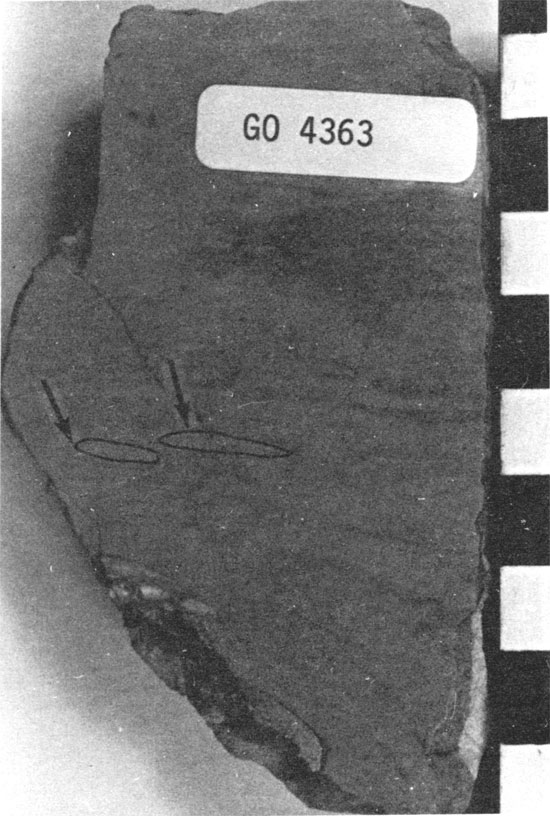
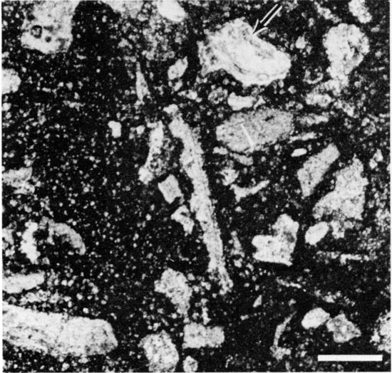
Figure 15--Photomicrograph of dolomitic intraclast wackestone facies of the upper cherty dolomitic limestone. Note the difference in grain size between the intraclasts (dark) and the matrix (light). The bar scale is 1 mm.
The dolomite consists of very fine- to coarse-grained subhedral to rhombic crystals. Larger rhombs display alternating layers of nonferroan and ferroan dolomite. Mudstones and wackestones may have laminations, with alternating layers of medium- and coarse-grained rhombs or very fine- and fine-grained subhedral crystals. Intraclasts may exceed 2 cm (0.79 inch) in length, are composed of very fine-grained dolomite, and tend to be more ferroan than the coarser grained matrix. The difference in crystal size in the laminations and between the intraclasts and matrix may represent variation in original size of sediment or, in the case of intraclasts, different times of dolomitization. The intraclasts, which are very fine grained, may have been penecontemporaneously dolomitized before transport, whereas the matrix was dolomitized in a later diagenetic event.
The crinoid packstone-grainstone facies of the basal limestone was unconformably deposited on the Simpson after a marine transgression. The facies represents deposition in a moderate to high-energy, open-marine environment with normal salinity. The fact that this unit thins to the northeast supports the idea of a gradual shallowing in this direction, which presumably continued throughout deposition of the Viola. Taylor (1947) proposed an unconformity at the top of the basal limestone in north-central Kansas; such an unconformity may occur in the study area, but cannot be documented conclusively.
Shaw (1964) stated that vertical successions of environments displayed in autochthonous rocks deposited in epeiric seas are reflections of a lateral sequence that existed at any given time. Accordingly, the mudstones at the base of the lower cherty dolomitic limestone represent an environment that was laterally equivalent to the crinoid packstone-grainstone facies over which the mudstones were deposited. The environment of deposition of the mudstones was in the lee of the crinoid packstone-grainstone facies. Conceivably, the mudstones were separated from the packstones and grainstones by a less restricted environment such as that which produced the mixed-skeletal wackestones which occur at the top of this unit.
In cores, the transition from the open-marine environment of the crinoid packs tone-grainstone facies to the very restricted environment of the mudstones is abrupt. The actual transition, however, is not represented in the cores. The abrupt change may reflect an unconformity, marine regression, or seafloor uplift that occurred after the deposition of the crinoid packstone-grainstone facies. The semirestricted mixed-skeletal wackestone facies which separated the open-marine crinoid packstone-grainstone facies from the very restricted mudstone facies is absent in the transition of the basal limestone to the overlying unit. Therefore, the possibility that the transition represents progradation of the restricted facies over the open-marine facies is unlikely.
The depositional environment of the mudstone facies was characterized by abnormal salinity or the absence of life-sustaining nutrients. Shaw (1964) postulated that because of presumed shallow slopes in epeiric seas, friction would have dampened the effects of normal, diurnal tides. Shallowness of the sea would have prevented the development of great nutrient-laden currents like those in modern oceans (Belak, 1980). Under such conditions, lack of adequate circulation would have created areas of increasing restriction as the sea shallowed toward the Central Kansas Arch. Excessive evaporation in this area, without replenishment with fresh waters, could result in the development of progressively higher salinities toward the arch, beyond the limits of tidal exchange. This model indicates an environment that is restricted through both a lack of life-sustaining nutrients and the presence of abnormally high salinity. In an alternative model, it is possible that the environment was characterized by abnormally low levels or seasonal fluctuations in salinity, caused by extensive influx of meteoric fresh water.
After the abrupt marine regression or sea floor uplift that preceded deposition of mudstones at the base of the lower cherty dolomitic limestone unit, a gradual marine transgression occurred, which resulted in the deposition of mixed-skeletal wackestones over the mudstones. The skeletal wackestones were deposited under semirestricted, low-energy conditions, probably between the depositional belt of the mudstone facies and that of the crinoid packstone-grainstone facies.
The marine transgression continued, culminating in the deposition of the crinoid packstone-grainstone facies of the upper limestone unit. During this period, moderate- to high-energy, open-water marine conditions again prevailed in the study area.
The deposition of the mixed-skeletal wackestones of the upper cherty dolomitic limestone unit over the crinoid packstone and grainstone of the upper limestone resulted from either progradation of facies belts seaward during a stillstand in sea level or development of the Pratt Anticline which forced the environments seaward. Whichever occurred, the depositional slope was probably steeper than it was during earlier deposition of the Viola, resulting in less restricted conditions behind the crinoid packstone-grainstone facies, and producing narrower depositional belts. The semirestricted, low-energy environment of deposition of the mixed-skeletal wackestones shallowed toward the Pratt Anticline. Shallow water restricted circulation, leading to the deposition of intraclast wackestone and laminated mudstones along the slopes of the anticline.
A generalized depositional model for the Viola in south-central Kansas is shown schematically in Figure 16, which summarizes lateral relationships between facies of the informal stratigraphic subdivisions. In this interpretation, the crinoid packstone-grainstone facies was deposited in an open-marine environment, the mixed-skeletal wackestones in a semirestricted environment, and the dolomitic mudstones deposited in a very restricted, low-energy environment. The facies belts roughly paralleled the Central Kansas Arch, which is located to the northeast of the model.
Figure 16--Generalized model for depositional environments in the Viola Limestone in south-central Kansas.
Following the deposition of the Viola, the sediments were subaerially exposed, resulting in an unconformable contact between the Viola and the Maquoketa Shale (Adkison, 1972).
Studies by Lee (1956), Merriam (1963), and Adkison (1972) concluded that the structural configuration of Kansas has remained virtually stable since the beginning of the Middle Pennsylvanian. Tectonic events that noticeably affected the Viola in south-central Kansas took place between the Middle Ordovician and the Middle Pennsylvanian. The first of these occurred after deposition of the St. Peter Sandstone (Lee, 1956). At this time the Central Kansas Arch began its development (Lee, 1943; Lee and others, 1946; Adkison, 1972). The continued uplift of this structural feature and the concomitant formation of the North Kansas Basin and the Southwest Kansas Basin, following deposition of the St. Peter, was intermittent and occurred during both periods of sedimentation and periods of emergence (Lee, 1956). This early structure influenced Viola deposition by restricting marine circulation because of shallowing in a northeast direction across the study area. The structure's influence on postdepositional diagenesis is indicated by the extensive dolomitization that occurred along the flanks of the arch after the Viola was uplifted into the mixed meteoric-marine zone.
Although Adkison (1972) considered formation of the Pratt Anticline to be mainly Early Pennsylvanian in timing, lithologic evidence in the study area suggests that it existed at least as a submerged high during deposition of the upper cherty dolomitic limestone. Further uplift before deposition of the Chattanooga Shale is strongly suggested by the extensive karst topography formed on the Viola and the contemporaneous development of the extensive Viola residual chert (Adkison, 1972).
According to Rutledge and Bryant (1937), the Cunningham Anticline, which extends from the southwest corner of Township 28 South, Range 11 West, to Township 26 South, Range 6 West formed at the time of the Wichita orogeny in the Early Pennsylvanian. Some of the most extensive dolomitization of the Viola in south-central Kansas is associated with this and the Willowdale Anticline (Merriam, 1963) in Township 29 South., Range 9 West, indicating that these structures formed either during or before dolomitization, perhaps beginning their upward movement even earlier than the Wichita orogeny. Also during Early Pennsylvanian time, fault-bounded blocks in Township 27 South, Range 13 West, T 29 S, R 14 W, and T 33 S, R 15 W were activated. These were named the Iuka horst, Coats horst, and Deerhead horst by Bornemann (1979). Dolomitization is not associated with these uplifted blocks. This implies that some dolomitization occurred between the time of formation of the Cunningham and the Willowdale anticlines and the block faulting of the horsts. Both of these events had ended by Early Pennsylvanian time and contribute to the structural grain of south-central Kansas, which exhibits trends striking generally northeast or southwest. These trends are thought to correspond to readjustments of tectonic trends in the Precambrian basement (Rich, 1933).
The cumulative result of these structural movements at various times was differential erosion and thinning of the Viola to the east within the study area. The recognition of four informal subdivisions of the Viola within cored wells in Barber and Pratt counties gave the key to their lateral correlation using the areal control provided by sample logs. The geographic disposition of the Viola subdivisions is summarized in the block diagram of Figure 17, which shows the gross lithologic composition of the Viola across the eastern half of the study area.
Figure 17--Block diagram of the eastern half of the study area showing the present distribution of the Viola subdivisions. Basal limestone = 1; lower cherty dolomitic limestone = 2; upper limestone = 3; upper cherty dolomitic limestone = 4.
Most wells in the study area were logged with a limited set of wireline logs. A typical logging program might consist of either a gamma ray or a spontaneous potential log, a single "porosity log" (either sonic, neutron, or density), and a resistivity log. Logs of Viola sections were digitized from 254 wells, whose locations are shown in Figure 18. The total sample consisted of 194 neutron, 62 sonic, and 36 density logs, in addition to gamma ray and resistivity traces.
Figure 18--Location of Viola well control in study area. Symbols on wells indicate a neutron • , sonic A density m , or two or more porosity logs *.
While a single "porosity log" is adequate in monominerallic rocks such as pure limestones, more complex lithologies require additional information for satisfactory porosity estimations. This problem usually has been resolved by simultaneously recording several porosity logs in sections of interest. Since each log measures a different physical property, their separate responses to different minerals allow a qualitative distinction of both mineral composition and pore volume. The choice of such an expanded logging program is appropriate for the Viola, since a typical section consists of interbedded limestones and cherty dolomites. However, the practice is a relatively recent innovation so that only a few wells in the area have been logged with neutron, density, and sonic tools.
One such well is Cities Service Belcher A-1 (C-NE-NE, 21-32S-17W), located in Comanche County to the west of the area evaluated in the core and cuttings study. Gamma ray, neutron, and density logs of the Viola section are shown in Figure 19. The neutron and density logs are overlaid on a common reference scale of porosity units which are calibrated with respect to a hypothetical limestone. In pure limestone intervals, the two traces should coincide on a common (and true) porosity reading. Appreciable amounts of either dolomite or shale cause the neutron log to record a higher apparent porosity value than the density log. Shales generally can be distinguished from dolomites by their higher gamma ray values. The influence of silica, either as sand or chert, is registered by a tendency for the density log to be drawn to higher porosity readings than is the neutron log.
Figure 19--Gamma ray, neutron, and density logs of the Viola Limestone in Belcher A-1 (21-32S-17W), Comanche County.
The application of these basic pattern recognition rules to the gamma ray, neutron, and density logs of the Belcher A-1 well yields a generalized impression of the variation in lithologies within the Viola. Detailed analysis Is obscured by compositional variations of calcite, dolomite, and chert, whose separate effects are compounded in a complex manner. Some of these ambiguities can be resolved by cross-plotting the porosity logs.
Within a single well, cross-plots may be made of porosity log readings of common depth zones as simple graphs, whose vertical and horizontal axes correspond to two porosity log scales. Since the theoretical values of pure sandstones, limestone, and dolomite are known for any range of porosity, these can be drawn on the cross-plot as a reference framework. The location of zone log coordinates identifies the zone compositions, both in terms of mineralogy and pore volume, by interpolation between these boundaries.
An example of a neutron-density frequency cross-plot is shown in Figure 20, which summarizes readings from the Viola in Belcher A-1. The general character of the frequency distribution suggests a variable mixture of limestones and dolomites with appreciable amounts of chert. The precise composition of any specific zone is somewhat ambiguous, since a slightly dolomitic limestone is difficult to distinguish from a cherty dolomite or a cherty dolomitic limestone. This ambiguity is caused by the restricted number of "knowns" (the porosity logs) relative to the number of "unknowns" (porosity plus mineral components).
Figure 20--Frequency cross-plot of neutron and density log responses from zones in the Viola of the Belcher A-1 well.
The uncertainties could be resolved by simultaneously plotting responses from three porosity logs (neutron, density, and sonic) along three axes, but such a presentation is difficult to visualize. The M-N plot was devised as an ingenious graphic solution of this three-dimensional problem, reducing it to two dimensions by the elimination of one of the unknowns (Burke, Campbell, and Schmidt, 1969). The composite variables M and N may be computed from pairs of porosity logs in a manner which suppresses the contribution made by the pore volume. The tetrahedron which links the end members of calcite, dolomite, quartz, and pore fluid is compressed onto the basal mineral composition triangle by a conical projection. This corresponds to a hypothetical view that would be seen by looking down on the tetrahedron from the fluid point.
An M-N plot of the Viola section in the Belcher A-1 well is shown in Figure 21. Although many zones plot within the compositional triangle of calcite-dolomite-quartz, a significant number plot outside the triangle. Some allowance must be made for errors introduced by poor log calibration and imprecise depth registration, but these external points are clearly influenced by additional systematic factors. The simplest interpretation for points which lie above the composition triangle is that the rocks contain coarse porosity such as vugs and fractures. The sonic log records the arrival time of the first acoustic wave and consequently is sensitive to the presence of small, intergranular and intercrystal line pores, but effectively "blind" to larger voids. The sonic estimation of porosity thus differs from estimates based on neutron and density logging devices which measure total pore volume. This difference in pore evaluation translates zones having an appreciable "secondary porosity" in a direction parallel to the M-axis. Most of these displaced points are drawn from the more cherty part of the composition triangle and can be readily equated with fractured cherty zones. Points which occur below the composition triangle are marked by high gamma ray readings, reflecting the influence of minor amounts of shale as an accessory component of the rock. The trend of these points is towards a hypothetical shale end member having low M and N values, closely matching the log characteristics of the underlying Simpson shales. The M-N plot therefore differentiates an internal mineral facies scheme of calcite, dolomite, and chert from external facies of fractured and vuggy cherty dolomites and shaly carbonates.
Figure 21--M-N plot of the Viola Limestone in the Belcher A-1 well. Φ N, Δt, ρb represent neutron, sonic, and density log readings of a zone. The subscript f designates hypothetical log readings for pore water.
Cross-plots are examples of mineral resolution by geometrical methods; these graphic results may be duplicated numerically by simple matrix algebra. In any depth zone, a measured log response may be partitioned among the contributions made by its component minerals and pore fluid by the equation:
where L is the log response,
n is the number of components,
vi is the proportion of the ith component, and
ai is the log coefficient associated with the ith component.
For example, when applied to the density log, the equation is a mass balance relationship which sums the fractional densities of the components into a composite bulk density. Analogous relationships for the neutron and sonic logs are linear approximations which have a reasonable match with physical models.
A combination of several log response equations may be written compactly in matrix algebra notation as:
L = AV
where L is a vector of log responses,
V is a vector of component proportions, and
A is a matrix of component log coefficients.
The coefficient matrix is augmented by the inclusion of a unity equation which expresses the closure of the system, so that the components collectively sum to one, or 100 percent. The vector of component proportions may be solved by the relationship:
V = A-1 L
where A-1 is the inverse of the coefficient matrix, A. When coded as a simple computer program, transforming wire-line logs into traces of mineral composition variation is straightforward. A coefficient matrix of the component log responses is compiled and inverted. The composition of any depth zone can then be evaluated by premultiplying the log readings of the zone by this inverse matrix.
A neutron-density-sonic logging suite is therefore sufficient to resolve four components in a matrix algebra solution. When applied to the Viola, compositions can be evaluated in terms of calcite, dolomite, chert, and pore fluid, and expressed in vertical profiles of variation. This type of presentation is an advance on the cross-plot where information concerning depth is lost. Some depth zones may produce irrational solutions of the component proportions; these coincide with anomalous points on the M-N plots. Zones with "negative proportions" of dolomite indicate the occurrence of residual chert; those with "negative proportions" of calcite indicate shaly carbonates.
An example of matrix algebra processing of the Viola section in the Belcher A-1 well is shown in Figure 22. The presentation differs from a conventional lithological log in showing a set of fluctuating traces rather than a sequence of discrete lithologies. A major reason for this difference is the vertical resolution of the porosity log combination which is on the order of a few f eet. This causes the compositional variation to be expressed as a smoothed moving average.
Figure 22--Mineralogical profile of the Viola Limestone in the Belcher A-1 well computed from logs using matrix algebra.
The Viola compositional profile in the Belcher A-1 well is not an end in itself, but rather contributes to interpretations of stratigraphy, mineral associations, depositional facies, diagenesis, and porosity development. Since logging data is intrinsically numerical, systematic analyses can be made of patterns and interrelationships by using statistics and signal theory.
The compositional variation of the Viola in this well in terms of the end members calcite, dolomite, and chert is shown in Figure 23. The calculation of a compositional trend summarizing the basic pattern of variation is complicated because the mineral percentages collectively describe a closed system. If the relative amounts of each of the three minerals are plotted along three orthogonal axes, all possible compositions are confined to a triangular plane (Fig. 24). Consequently, the three apparent dimensions of the system are really described by two axes in a plane.
Figure 23--Composition triangle of zones from the Viola of the Belcher A-1 well.
Figure 24--Graphic demonstration of system closure for compositional variables which shows that all possible mixtures of three end members are confined to a two-dimensional composition plane.
The coordinates of compositions lying on this plane may be calculated by a Helmert transformation:
z1 = (y2 - y1) / √2
and
z2 = (2y3 - y1 - y2)/√6
where y1, Y2, Y3 are the proportions of calcite, dolomite, and chert, and zl, z2 are the transformed planar coordinates. A reduced major axis was fitted to the transformed compositional data as a line of best fit (Fig. 25). This shows a basic trend in composition ranging between two end members, limestone and cherty dolomite. The trend matches the observational data from core and cuttings,
Figure 25--Reduced major axis computed as a best fit trend of compositional variation of the Viola Limestone zones in the Belcher A-1 well.
Trends in porosity variation with respect to compositional variation were mapped by regression analysis. The equation for a linear trend is given by:
and describes a best-fit plane of the trend in porosity (![]() ) which crosses the compositional triangle. This linear surface (Fig. 26) has a fit of only 4 percent to the raw porosity data. However, it is statistically significant at the 95-percent level and shows a general increase in porosity with increasing dolomite content.
) which crosses the compositional triangle. This linear surface (Fig. 26) has a fit of only 4 percent to the raw porosity data. However, it is statistically significant at the 95-percent level and shows a general increase in porosity with increasing dolomite content.
Figure 26--Linear trend surface of porosity variation in the Viola Limestone of the Belcher A-1 well, computed as a function of calcite, dolomite, and chert content.
The equation for a quadratic (or second-order) trend is:
which provides a markedly improved estimate of porosity variation with a fit of 31 percent (Fig. 27). This is a statistically significant improvement over the linear trend. Porosity in low-porosity limestones gradually increases towards the chert end member; this increase is probably caused, at least in part, by vugs and fractures in the cherty limestones. The relatively low porosities of highly cherty dolomites may reflect the influence of small amounts of argillaceous material in this facies which reduces the overall porosity. The marked increase in porosity moving from the limestone to dolomite compositional field is readily explained in terms of original depositional facies and subsequent diagenesis. Core analysis shows that the limestones are crinoidal packstones and grainstones in which pore volumes have been partially occluded by syntaxial overgrowths of calcite. In contrast, dolomites are wackestones whose high porosities probably were a causative factor in their selective dolomitization.
Figure 27--Quadratic trend surface of porosity variation in the Viola Limestone of the Belcher A-1 well, computed as a function of calcite, dolomite, and chert content.
Time series of fluctuating data, such as economic indices or meteorological variables, often are fitted by polynomial functions of time to distinguish long-term trends from local fluctuations. This approach can be used to analyze variation in estimated calcite content within the Viola as a function of depth. Any systematic trends which are extracted should reflect major stratigraphic patterns of the disposition of limestone and cherty dolomite facies.
A first-order polynomial takes the form:
where ![]() is the trend value of the calcite content and d is the depth, in an equation which defines a straight line. The second-order polynomial is:
is the trend value of the calcite content and d is the depth, in an equation which defines a straight line. The second-order polynomial is:
and describes a parabola, a curve with a single maximum or minimum. The general equation of an nth-order polynomial is:
which will have (n-1) maxima and minima and (n-2) inflection points, expressing peaks and troughs and boundaries between them, respectively,
Each equation is fitted by the principle of least-squares deviation, which minimizes the variation about the trend. The degree of fit improves with increasing complexity of the polynomial equation and can be measured by the proportion of the total variation satisfied by the polynomial. A graph of polynomial fit against polynomial order reflects any major "natural" subdivision of the calcite profile (Fig. 28). A fundamental subdivision appears to be located by a fourth-order polynomial, since there is both a marked decline in the rate of improvement in fit by higher orders and an analysis of variance identifies the fourth order as the statistically most significant trend.
Figure 28--Graph of percent fit versus order of polynomial curve functions of calcite content regressed on depth in the Viola of the Belcher A-1 well.
This graphic polynomial trend is superimposed on the Viola raw calcite variation in Figure 29 and defines five basic stratigraphic subdivisions. The lower four are readily identified with the informal units recognized from core studies in the eastern part of the area: the basal limestone, the lower cherty dolomitic limestone, the upper limestone, and the upper cherty dolomitic limestone. Since the Belcher A-1 well is located in the west where the Viola is thicker, it appears that the uppermost unit represents a third limestone which overlies the upper cherty dolomitic limestone,
Figure 29--Calcite composition variation of the Viola Limestone in the Belcher A-1 well overlain by a fourth-order polynomial regression curve and indexed with Viola subdivisions.
Both the trend and variation of estimated calcite content in this Viola section give a valuable insight of the character of vertical (and, by implication, lateral) changes in lithofacies. Boundaries between the facies units show gradual transitions which appear to reflect long-term waxing and waning of calcite packstones and grainstones and dolomitized wackestones in the lateral migration of facies across the area. At a smaller scale, the boundaries between individual beds of these two facies appear to be fairly sharp.
The subtraction of the polynomial trend from the original data isolates the residual variation which represents relatively short-term facies changes. It is interesting to speculate whether the pattern of these residuals is random, or if it is described by some type of periodic component. A random nature would imply that individual limestone and dolomite beds represented chance local oscillations of facies which were subordinate to the major migrations of the facies belts recognized in the informal stratigraphic subdivisions of the Viola. Alternatively, a systematic periodic component would suggest a cyclic mechanism of depositional facies control.
Cyclic components in a sequence can be resolved by Fourier analysis, which translates the original variation in the time or spatial domain to a spectral representation in the frequency domain. The mathematical process is analogous to the manner in which a prism breaks white light into its colored components as a spectrum of different frequencies. One of the conditions of Fourier analysis is that the input data should be stationary, with no long-term drift or trend in average value. The fourth-order polynomial fitted to the calcite data is an expression of long-term variation, while the residuals retain information on short-term fluctuations and are effectively stationary.
The power spectrum of the calcite residuals (Fig. 30) is marked by a pronounced peak at approximately 20 feet, with harmonics at 10- and 5-foot wavelengths. The most common explanation for harmonic generation is that it results from a non-sinusoidal character of the fundamental frequency (Mackay, 1973). This effect could be caused by distinctive interbedding of limestones and cherty dolomites, where calcite variation would more closely follow a square-wave rather than a sine-wave pattern.
Figure 30--Power spectrum of residuals of a fourth-order polynomial regression fitted to calcite variation in the Viola Limestone of the Belcher A-1.
The power spectrum clearly indicates a periodic structure in the alternation of facies units within the informal stratigraphic subdivisions. The subdivisions probably represent the regional migration of facies belts as a consequence of some mechanism such as eustatic changes in sea level or platform subsidence. The presence of an internal cyclic pattern indicates that the process was not abruptly episodic, but continuous and oscillatory. From this interpretation, it follows that divisions that can be correlated over the region represent trends in either a major transgressive or regressive phase which are perturbed by minor reversals, and that the whole process has a distinctive cyclic character.
Cyclic variations in lithofacies and faunal distributions within the Ordovician are most commonly attributed to eustatic changes in sea level. So, for example, Sweet (1979) traced inflection points on relative-abundance diagrams of interpreted shallow- and deep-water conodont taxa in an attempt to define correlative sea level cycles.
In Late Ordovician (post-Viola) times, lithofacies variations in the Appalachian Queenston Delta have been linked directly with a glacial control of sea level (Dennison, 1976). Extensive late Ordovician glaciation has been recorded in northern Africa, southern Spain, Argentina, Peru, and Bolivia. The south pole appears to have been situated in Morocco, and it is here that the glacial maximum has been dated at the American time equivalent of the Richmond Stage of the Cincinnatian Series.
The influence of polar ice-cap fluctuations at an earlier time is more speculative, but has been invoked to explain sedimentary cycles in the Middle Ordovician Trenton limestone of southern Ontario by Brookfield (1982).
It is widely recognized that many logs have appreciable errors in calibration which need correction for accurate reservoir analysis. However, all logs are in error to some degree. Even after the most comprehensive environmental corrections, a log trace still includes error which is compounded from tool malfunctions, shop and field miscalibrations, and operator error. Such errors are a fact of life which applies to all physical measurements, whether made in the subsurface by logging tools, or the laboratory using the most sophisticated instruments. Logging errors are a nuisance factor in the estimation of accurate porosities, but may be a major problem in computing mineral proportions, since the log responses of quartz, calcite, and dolomite are very similar. The analysis of lithofacies from logs therefore requires remedial methods to screen out measurement errors.
Procedures which attempt to eliminate logging measurement errors usually are referred to as "normalization" or "quality control." Two excellent papers by Neinast and Knox (1973) and Patchett and Coalson (1980) review approaches to the art of normalization and discuss the merits and drawbacks of each technique. This report describes a new method for log normalization, which is a logical extension of earlier work.
Corrective shifts may be applied to log traces if readings can be referenced to a "calibration unit" or subsurface horizon with a constant log response over the area of interest. An example of an ideal calibration unit is a pure anhydrite bed, since anhydrite has distinctive and predefined physical properties. More commonly, a more pragmatic decision must be made concerning a suitable calibration unit. Certain shales or relatively tight carbonate horizons often are selected because they can be correlated over a wide area and their physical properties appear to vary only slightly. While not precisely constant, their log responses are at least "consistent."
The notion of consistency has intrinsic problems. All lithologies show some degree of variation in composition and texture. As a result, there is no unique value that is representative of the log response of even a well-chosen calibration unit, but, hopefully, the response will be restricted to a narrow range of variation. Changes in calibration unit properties will be linked with geography, reflecting a combination of changes in depositional facies, diagenesis, and compaction linked with structural position. This results in a geographic drift of the properties of the calibration unit, introducing a bias in the calibration of any log according to the location of the well.
To a certain extent, systematic geographic effects can be compensated for by the procedure suggested by Neinast and Knox (1973). They state that "daisy-chain circles are used from a base map to cross-check the possibility of normalizing gradual formation changes instead of tool variation." However, trend surface analysis may be used to monitor automatically any systematic geographic variation, and provides a simple and powerful predictive model for log calibration (Doveton and Bornemann, 1981).
If a variable Z is measured at locations with geographic coordinates X and Y. a smooth surface may be fitted through the Z values which will express the regional trend in Z. The simplest example of a trend surface is a linear (or first-order) trend, given by the equation:
where ![]() is the value of the trend surface at location X, Y and a, b, c are constants. The equation describes a plane which can be fitted to the observations of Z by the criterion of least squares deviation (Fig. 31). The plane is positioned such that the sum of the squared deviations of Z from the plane is the minimum possible. Rather than find the orientation of the plane by a cumbersome trial-and-error method, the equation may be solved directly by simple matrix algebra programmed on a computer.
is the value of the trend surface at location X, Y and a, b, c are constants. The equation describes a plane which can be fitted to the observations of Z by the criterion of least squares deviation (Fig. 31). The plane is positioned such that the sum of the squared deviations of Z from the plane is the minimum possible. Rather than find the orientation of the plane by a cumbersome trial-and-error method, the equation may be solved directly by simple matrix algebra programmed on a computer.
Figure 31--Hypothetical trend surface plane fitted to observational data Z, measured at geographic locations X and Y.
The linear surface is the most basic member of a sequence of polynomial trend surfaces which can be fitted to observational data. The quadratic (or second-order) surface is given by:
and represents a curved surface which can have the form of a dome, basin, or saddle. Successively more complex surfaces can be generated by adding higher powers of X, Y, and their cross-products. However, in all instances, the solution of their descriptive equations follows the same matrix algebra procedure, but with an expansion of the number of terms and the size of the matrices.
Since a series of possible trend surfaces may be computed, the most appropriate surface to use for the problem at hand must be selected. At one extreme, it is possible to compute a trend surface which is so complex that it precisely fits all the observation points. At the other extreme, a very simple surface may not be a good representation of the regional pattern (for example, a plane may be fitted to a surface which actually has the shape of a dome). Each trend surface accounts for a proportion of the total variation in the data, calculated as the degree of fit. By comparing the fits for a sequence of trend surfaces, it may be possible to identify a polynomial order which defines a major regional trend, when higher orders provide only minor increases in fit. Alternatively, this assessment may be made more rigorously by statistical inference, testing to determine if the next highest order of trend surface provides a significant improvement in fit over the previous surface.
The theoretical model behind trend surfaces is linear regression analysis, which partitions the total variation of the data into a broad systematic component representing large-scale geographic variation and into a residual component. When applied to the log response of a calibration unit, the trend surface procedure extracts any systematic geographic drift in variation, while the deviations of the data from the surface are estimates of the measurement error. If the appropriate model has been selected for the trend surface, the residuals should represent normally distributed errors about the surface and should show no spatial (geographic) correlation.
A trend surface may be used both to normalize logs in existing wells and to predict normalized calibration unit values at prospective drill sites. The correct value of the calibration unit is estimated by inserting the geographic coordinates of the location of interest into the trend surface equation. In addition, a histogram of the deviations of the observations from the surface shows the distribution of tool errors in the area, as well as any systematic local effects. Prognosis (the trend surface) and diagnosis (the residuals) are the two major functions of this trend surface application.
The basal limestone is essentially a pure limestone with only minor amounts of chert and dolomite, and porosity appears to be restricted over a range of 3 percent. The simple mineralogy, moderately uniform porosity, and absence of hydrocarbons suggest that it is a reasonable choice for a log calibration unit. Data were drawn from 254 wells which penetrated the Viola and were logged by at least one porosity tool. Porosity logs were digitized over the range of the Viola; the total sample consisted of 194 neutron, 62 sonic, and 36 density logs. In each well, average neutron porosity, transit time, and density readings were calculated for the basal limestone, excluding the upper and lower 2 feet of the unit to minimize the effect of adjacent beds. The three sets of neutron, sonic, and density readings were independently studied by trend surface analysis.
Linear, quadratic, and cubic trend surfaces calculated for the basal limestone neutron data have fits of 6.72, 12.01, and 13.49 percent of the total variation. These figures may seem depressingly low, but they are an indication that the basal limestone is a good choice as a calibration unit. If the fits were high, the trend surfaces would imply that there was a major drift in the calibration standard across the area.
The degree of fit of the quadratic surface is almost double that of the linear surface, but the cubic is only a minor improvement on the quadratic. The quadratic surface thus appears to be the best expression of systematic regional variation of the basal limestone neutron response. This interpretation was checked by an analysis of variance test of whether successively higher orders of surface make a statistically significant improvement over lower orders (Table 2). The linear surface is significantly better for predicting the neutron response of the basal limestone at any location when compared to use of the average neutron response in the data set. This demonstrates that trend surface analysis has detected a systematic geographic variation in the calibration unit. The quadratic surface provides a significant improvement in fit over the linear, but the cubic fails to add significantly to the quadratic.
Table 2--Analysis-of-variance table of trend surfaces fit to the basal limestone neutron data. Asterisks indicate F-ratios significant at the 95-percent level.
| Source of Variation |
Sum of Squares | DF | Mean Squares |
F-Ratio |
|---|---|---|---|---|
| Linear regression | 27.22 | 2 | 13.61 | 5.73* |
| Linear deviation | 377.62 | 159 | 2.37 | |
| Quadratic-linear regression |
21.41 | 3 | 7.14 | 3.13* |
| Quadratic deviation | 356.22 | 156 | 2.28 | |
| Cubic-quadratic regression |
5.99 | 4 | 1.50 | 0.65 |
| Cubic deviation | 350.23 | 152 | 2.30 | |
| Total variation | 404.85 | 161 |
The quadratic trend surface shown in Figure 32 indicates a broad central area of relatively high porosity flanked by lower porosities to the west and southeast. It is worthwhile to relate log response trend surfaces with regional geology patterns in order to assign meaning to the trends and to crosscheck their validity. The quadratic surface shows a striking concordance with the axis of the Pratt Anticline (Fig. 1) and suggests a genetic relationship between the two. St. Clair (1981) detected facies changes in the upper cherty dolomitic limestone unit, from mixed-skeletal wackestones to intraclast wackestones and laminated mudstones on the flank of the Pratt Anticline. The neutron trend surface indicates that the Pratt Anticline was an active positive feature as early as the time of deposition of the basal limestone. The trend in porosity may reflect a regional pattern of low porosity, grain-supported crinoidal packstones and grainstones on the margins of the Pratt Anticline, which grade toward the anticlinal axis into a slightly more micritic and more porous lateral equivalent.
Figure 32--Quadratic trend surface of basal limestone neutron porosity variation expressed in limestone porosity units.
Trend surfaces were computed for transit times and densities of the basal limestone and in both instances the linear surface was found to be most significant for portraying the regional variation of the data. A contour map of the transit time linear surface (Fig. 33) shows a simple decline in porosity, moving from the northeast to the southwest, which is only a general approximation of the trend in the neutron data. A major reason for this difference is that the sample of sonic logs contains fewer than one-third the number of neutron logs. The small sample size is not large enough to pick up any systematic improvement by the quadratic surface.
Figure 33--Linear trend surface of basal limestone transit time variation (microseconds per foot).
The same argument applies to the linear surface of density where the sample consists of only 36 wells. However, the linear surface of density (Fig. 34) shows a decline in porosity to the east which seems to contradict the trends in both neutron and sonic properties. The apparent discrepancy is explained by the distribution of the wells having density logs, which are restricted almost entirely to the eastern half of the area. The surface of density measurement is therefore primarily sensitive to the decrease in porosity on the eastern flank of the regional structure. This illustrates the important point that trend surface predictions of calibration unit response must be confined to areas of moderate well control and not extrapolated beyond these limits.
Figure 34--Linear trend surface of basal limestone bulk density variation (grams per cubic centimeter).
While the trend surfaces of the basal limestone porosity values are estimates of systematic regional variation, deviations of values from the surface can be attributed to tool error and any systematic local variation. If the residuals are the result of tool error alone, they should be approximately normally distributed with a mode located at zero. Frequency polygons of the neutron, sonic, and density residuals are shown in Figure 35, plotted on a compatible scale of limestone porosity units. Each distribution shows a slight positive skew with the modal peak displaced to approximately -1 porosity units. This implies that the true variation of the basal limestone closely follows the form of the trend surfaces, but local areas have either the development of enhanced porosity zones or increased shale content. As a result, the trend surface estimates will tend to be slightly high over most of the area by about 1 porosity unit, but in local areas may be low by approximately 2 porosity units. Following conventional practice, each trend surface equation can be modified by subtracting the displacement of the mode from zero and inserting this quantity as a correction factor. The modified equation now reflects the most typical values for the area, rather than the arithmetic average. Potential areas of problems caused by enhanced porosity can be determined from contour maps of the residuals, although it may be difficult to distinguish these from spurious features caused by positive tool errors.
Figure 35--Frequency polygons of basal limestone neutron, sonic, and density trend surface residuals.
Analysis of both the trend surfaces and their associated residuals provides useful feedback concerning the utility of the basal limestone as a satisfactory calibration unit, as well as numerical relationships for prediction and control. Simple descriptive statistics and inferential tests may be systematically applied to dissect log quality in the area if the residuals can be reasonably approximated by normal distributions. The area under the curve of a normal distribution is a function of a scale of standard deviations about the mean and dictates the proportion of tool errors to be expected within specified ranges. So, for example, if an accuracy of +1 or -1 porosity unit is considered an acceptable tolerance level, 49 percent of the neutron logs will require correction, since the standard deviation of the neutron log is 1.51 porosity units. Similarly, 69 percent of both sonic and density logs will require correction.
From trend surface analysis, predictive equations were developed to normalize all porosity logs in the area, including those of the Belcher A-1 well. This remedial operation is a necessary preliminary step in the mapping of lithofacies of the Viola from logs.
Mapping of changes in lithology across an area requires an extension of the method developed for characterization of individual well profiles to a form suitable for lateral interpolation. In theory, it would be possible to compute compositional profiles of the Viola at each well location, calculate average compositions, and use the results as input for a mapping procedure. However, the Viola data set, in common with most other studies of this type, has a severe deficiency. Only two wells in the entire sample have a complete neutron-density-sonic log combination. in the majority of wells, only one porosity log was run, so a new approach to the problem must be devised.
If a porosity log suite in a stratigraphic unit can be transformed into a compositional profile, the mean composition of the unit is readily calculated by averaging the total vertical variation. An identical result can be obtained by directly transforming the average log responses of the unit. This equivalence implies that in order to compute the unit mean composition at any location, the average log responses of the unit are required rather than a complete suite of log traces.
Average log responses of a major stratigraphic unit will change gradually when traced laterally between wells, so these variations can be regarded as continuous hypothetical surfaces across the area. Such surfaces can be approximated, using computer mapping packages, as grids of numerical values. Grid rows and columns specify geographic position, while the grid node values are estimated by interpolation from available well control data. On this basis, three surfaces of average Viola neutron, density, and sonic log responses may be computed independently as grids drawn from the separate sets of control logs. The three grids can be generated over the entire study area in a manner so that an estimated average response of each porosity log is available at all geographic locations specified by the grid nodes.
The normalized Viola average log responses were used as input to an automated contouring program in the generation of grids for neutron, density, and sonic values. The matrix algebra method described for the analysis of vertical variation was extended to the transformation of these log response grids to compositional grids of calcite, dolomite, chert, and porosity proportions. Rather than convert a sequence of depth zone log responses to compositional profiles, the procedure was modified as a grid-to-grid operation in which corresponding grid nodes were successively transformed.
Grid node proportions were plotted with reference to a calcite-dolomite-chert composition triangle (Fig. 36). This ternary diagram is highly unconventional, as many of the grid nodes are associated with negative fractions of components. These anomalous points can be simply explained by comparison with the M-N plot of Figure 21. Points which lie above the calcite end member indicate systematic coarse porosity which generally is associated with residual chert and weathered carbonate. Points below the dolomite-chert line reflect the influence of minor amounts of shale as an additional component. Following this line of interpretation, the diagram was subdivided into six lithofacies types. The calcite-dolomite-chert triangle was allocated between three facies of limestone, dolomite, and chert, determined by the dominance of one of the three minerals. The remainder of the diagram was divided into three lithofacies equated to residual chert with carbonate, carbonate with residual chert, and shaly carbonate.
Figure 36--Ternary diagram of computed mineral percentages at map grid nodes, indexed with lithofacies subdivisions.
The lithofacies subdivision of the diagram allowed the four grids of compositional variation to be combined into a single lithofacies representation, in which each set of grid nodes could be allocated to one or other of the six lithofacies. The result is shown in Figure 37 and Plate 1, where the size of the grid cells conforms approximately to the average density of well control in the area.
Figure 37--Petrophysical lithofacies map of the Viola Limestone.
The structural map of the top of the Viola (Fig. 38 and Plate 1) shows details of the major structural features shown on the regional map of Figure 1. To the north of the area, the southern limit of the Central Kansas Uplift is linked with the Pratt Anticline which marks a boundary between the Hugoton Embayment to the west and the Sedgwick Basin to the east. Structure contours in the eastern half of the area show a marked NNE grain of localized features which persist to the Precambrian basement. This character was observed by Rich (1930) who was "at once struck by the pronounced rectangular pattern of the structure and . . . that the area seems to be divided into blocks bounded by nearly straight sides, or fracture lines." In a discussion of seismic anomalies on the Pratt Anticline, Brewer (1959) suspected faulting and differential erosion of Lower Paleozoic rocks.
Figure 38--Structural elevation map of the top of the Viola Limestone (meters subsea).
The isopach map of the Viola (Fig. 39) shows a regional trend of increasing thickness to the west which is confounded by significant local variations. It is probable that the depositional thickness of the Viola increased in a southwesterly direction away from the Central Kansas Uplift, and would mirror a similar trend in the Viola in the Salina Basin to the north of the Chautauqua Arch (Taylor, 1947). Regional uplift that preceded deposition of the Late Devonian Chattanooga Shale probably was responsible for the westerly orientation of gross thickness trends as differential erosion modified the earlier depositional trend.
Figure 39--Isopach map of the Viola Limestone (meters).
The second major tectonic event began its major cycle of activity in the Late Mississippian and culminated in the Early Pennsylvanian (Lee, 1956; Merriam, 1963). Its effect on the Viola was categorically different from earlier tectonic uplift. While uplift caused differential erosion of the Viola and determined regional thickness variation in the formation, the second event finalized the structural configuration of the area. The present disposition of the Pratt Anticline was established and fault-bounded blocks were activated in the east so that Pennsylvanian erosion reached the Viola Limestone and caused additional thinning over these features and created marked topographic relief.
The influence of these tectonic events can be seen on the Viola lithofacies map based on well logs. The facies interpreted as "residual chert" forms a belt which borders the Central Kansas Uplift to the north and parallels the subcrop of the Viola. The extension of this facies to the south, together with isolated outliers, reflects the trend of the Pratt Anticline. This petrophysical interpretation accords well with a map of residual chert thickness determined from cutting logs by Adkison (1972). The chert regolith resulted from extensive weathering in the Late Devonian, Late Mississippian, and Early Pennsylvanian.
The facies designated as "carbonate with subsidiary residual chert" is located mainly in the center of the area and has an intimate association with the "residual chert facies." Several sample logs in this facies area report thin developments of shale and sandstone which are similar to those of underlying Kinderhookian rocks. One well (G.M.R. 2 Betzer, 34-29S-16W) shows 46 feet (14 meters) of "intra-Viola detritus" as a jumble of Viola chert and dolomite in clay and shale, which is overlain by shale and cherty clay. Adkison (1972) has suggested that "some of the non-carbonate clastic deposits are probably misidentified cavern fillings of post-Viola age." If this interpretation is correct, the two residual facies of "residual chert with carbonate" and "carbonate with residual chert" are paleogeomorphic, the former representing a detritus regolith and the latter karstic solution-weathered carbonates.
A map of representative cuttings from the area is shown in Figure 40. These were selected from the open-file reports of a single geologist (J.D. Davies) in order to preclude differences in style. The arrangement of profiles of rock types generally agrees with petrophysical facies patterns and picks up the central limestone facies which grades outwards to dolomite. The "shaly carbonate" facies can be identified as cherty dolomite. The slightly "argillaceous" character of dolomites in these areas accounts for its shaly aspect as perceived by the logs, which are particularly sensitive to shale content.
Figure 40--Representative cuttings logs of the Viola. The location of each associated well is at the center of the strip. Key to lithologies: regular brick = limestone; oblique brick = dolomite; mixed brick dolomitic limestone; open triangles = bedded chert; closed triangles = residual chert.
The combined effects of depositional facies patterns and subsequent erosional bevelling of the Viola (summarized in Fig. 17) is the key that explains the regional disposition of "dolomite" and "limestone" facies on the log analysis map. A central limestone facies trending NW-SE is flanked by dolomite to the northeast and southwest. Because it is a composite analysis of the entire Viola section, the petrophysical facies will tend to reflect the dominance of the subdivisions. To the west, all four units are present and, since the dolomitized units are thicker than the limestone units, a composite facies of dolomite is determined. In the central region, the upper dolomite is absent, so the combination of both limestone units with the lower dolomitized unit results in a "limestone facies.11 To the east, only the thinner basal limestone and thicker lower dolomitized unit are present so the net effect is a "dolomite facies."
The petrophysical facies map exhibits a marked grain, with a lineation approximately NNE-SSW and NW-SE. This characteristic is most pronounced on contour maps of individual components. A contour map generated from the grid of chert proportion (bedded chert facies, rather than residual chert) is shown in Figure 41. The linear aspect can be related to features on both structure and isopach maps, and can be traced to the Precambrian basement. The history of these structural elements has been described earlier; they appear to represent ancient zones of weakness which have been reactivated at various times.
Figure 41--Contour map of Viola chert proportion (bedded chert facies) drawn from log analysis. Proportions greater than 0.2 are shaded.
One possible explanation for localized increases of chert in the vicinity of these tectonic features is through generation of chert by hydrothermal solutions in fracture systems. This genetic form of chert has been designated "T-chert" and its more localized concentrations would contrast with the normal bedded and nodular "S-chert" which can be attributed to regional mechanisms of diagenesis (Dunbar and Rodgers, 1957, p. 248). Alternatively, the uplift on block features associated with these anomalies may have caused extended residence times of the local Viola in phreatic mixing zones, which resulted in more extensive chert formation than normal.
Another explanation for this linear pattern is provided by the recent aeromagnetic survey of Kansas (Yarger, 1983). The relative total intensity magnetic field map of the area (Fig. 42) is singularly bland. However, the second vertical derivative of such data is sensitive to abrupt changes in magnetic susceptibility (Vacquier and others, 1951), measuring the rate of change in slope of magnetic field intensity. A second-derivative map (Fig. 43) shows a distinctive lineation which accords with the grain seen on both structural and petrophysical facies maps. These lineations are even more striking on second-derivative maps of the entire state (Fig. 44), where they represent features of regional significance. The NNE-SSW trends in the eastern half of the area appear to be southerly continuations of linear elements linked with the gravity and magnetic anomalies associated with the Proterozoic Central North American Rift System (CNARS). In the north of Kansas and beyond, the CNARS is marked by a pronounced gravity anomaly which probably represents an aborted "oceanic" rift in Precambrian times which is floored by Keweenawan mafic rocks (King and Zietz, 1971). The southern Kansas extension does not seem to have moved beyond an early period of block faulting and possible dike intrusion (Yarger, 1981). In summary, it appears that the study area straddles the western margin of an ancient rift system which has been intermittently active throughout geological time and whose effects can be perceived in lithofacies patterns derived from well logs. Indeed, these zones of weakness are still active, since four microearthquakes were recorded in the southeastern part of the area over a recent 3-year period (Steeples, 1982).
Figure 42--Relative total intensity magnetic field map of study area in gamma units (after Yarger, 1983).
Figure 43--Second-derivative map of relative magnetic field intensity in study area (after Yarger, 1983).
Figure 44--Second-derivative map of relative magnetic field intensity in Kansas (after Yarger, 1983).
The location of Viola oil fields is shown superimposed over a regional map of porosity, contoured from the grid of pore volume component that was generated as an intermediate step in the production of the lithofacies map (Fig. 45). Northeasterly trends can be seen which presumably were influenced by the tectonic elements and their history of preferential uplift, and the subsequent pattern of depositional facies, diagenesis, and erosion. Structural highs associated with porosities in excess of 7 percent are favorable for oil accumulation within the Viola. In areas where the Viola is thin and residual chert is absent, reservoirs are rare, probably because the formation has been stripped by erosion down to relatively tight, well-cemented calcite grainstones at the base.
Figure 45--Average porosity of the Viola from log analysis, indexed with Viola oil and gas fields shown by stippled patterns.
Systematic exploration in the area would obviously be aided by lithofacies and component maps from well logs in conjunction with more conventional structure and isopach maps.
Traditional use of wireline logs has been restricted to either stratigraphic correlation or the analysis of porosity and hydrocarbon saturations. Recent advances in log analysis have produced alternative methods for interpretation of lithofacies, which may enhance significantly the information obtained from cuttings and cores. The numerical form of logging data makes it particularly amenable to computer processing and the rapid production of compositional profiles and maps. The petrophysical analysis of logs may be viewed as a form of remote sensing in which "ground truth" supplied by more orthodox geological methods provides both the necessary control for validation, and the essential meaning of the observed patterns of variation.
In a study of the Viola Limestone of south-central Kansas, an integrated analysis yields the following conclusions:
The authors are indebted to a number of individuals for their help in various phases of this project. Drs. C.D. Conley, M.). Brady, and W.J. Ebanks, Jr. contributed to discussions on carbonate rocks and subsurface geology. Harold Cable, Jim Deputy, and Charles Ross assisted with programming problems, and Chris Roche and Joe Brentano produced the computer plots. We are also grateful to Dr. M.J. McCullagh for use of his computer contouring package. Pat St. Clair thanks Marathon Oil Company for their photographic work and Marvin Woody for his editorial work and moral support. Dr. J.C. Davis edited the final manuscript and JoAnne DeGraffenreid designed and prepared the camera-ready copy for printing.
Adkison, W.L., 1972, Stratigraphy and structure of Middle and Upper Ordovician rocks in the Sedgwick Basin and adjacent areas, south-central Kansas: U.S. Geol. Survey, Prof. Paper 702, 33 p. [available online]
Bathurst, R.G.C., 1966, Boring algae, micritic envelopes and lithification of molluscan biosparites: Geol. Jour., v. 5, p. 15-32.
Belak, R., 1980, The Cobleskill and Akron members of the Rondout Formation Late Silurian carbonate shelf sedimentation in the Appalachian Basin, New York State: Jour. Sed. Petrology, v. 50, p. 1187-1204.
Berry, W.B.N., and Boucot, A.J., 1970, Correlation of the North American Silurian rocks: Geol. Soc. America, Spec. Paper 141, p. 1-289.
Bornemann, E., 1979, Well log analysis as a tool for lithofacies determination in the Viola Limestone (Ordovician) of south-central Kansas: Unpub. Ph.D. dissertation, Syracuse University, 151 p.
Brewer, J.E., 1959, Geophysical problems on Pratt Anticline: Kansas Geol. Survey, Bull. 137, p. 275-280.
Brookfield, M.E., 1982, Glacio-eustatic sedimentary cycles in Trenton limestone (Middle Ordovician) of southern Ontario (abs.): Am. Assoc. Petroleum Geologists, Bull., v. 66, no. 8, p. 1165.
Burke, J.A., Campbell, R.L., Jr., and Schmidt, A.W., 1969, The lithoporosity crossplot: SPWLA Tenth Annual Logging Symposium Transactions, Y, p. 1-29.
Cloud, P.E., 1962, Environment of calcium carbonate deposition west of Andros Island, Bahamas: U.S. Geol. Survey, Prof. Paper 350, 138 p. [available online]
Dennison, J.M., 1976, Appalachian Queenston delta related to eustatic sea-level drop accompanying late Ordovician glaciation centered in Africa; in, The Ordovician System, M.G. Bassett, ed.: Proc. Paleont. Assoc., p. 107-120.
Doveton, J. H., and Bornemann, E., 1981, Log normalization by trend surface analysis: The Log Analyst, v. XXII, no. 4, p. 3-8.
Dunbar, C.O., and Rodgers., J., 1957, Principles of Stratigraphy: John Wiley, New York, 356 p.
Irwin, M.L., 1965, General theory of epeiric clear water sedimentation: Am. Assoc. Petroleum Geologists, Bull., v. 49, p. 455-459.
Jewett, J.M., 1951, Geologic structures in Kansas: Kansas Geol. Survey, Bull. 90, pt.. 6, p. 105-172. [available online]
King, E.R.., and Zietz, I., 1971, Aeromagnetic study of the Midcontinent gravity high of central United States: Geol. Soc. America, Bull., v. 82, p. 2187-2208.
Lee, W., 1943, The stratigraphy and structural development of the Forest City Basin in Kansas: Kansas Geol. Survey, Bull. 51, p. 1-142. [available online]
Lee, W., 1956, Stratigraphy and structural development of the Salina Basin area: Kansas Geol. Survey, Bull. 121, 167 p. [available online]
Lee, W., Grohskopf, J.G., Reed. E.L., and Hershey., H.G., 1946, The structural development of the Forest City Basin in Missouri, Kansas, Iowa, and Nebraska: U.S. Geol. Survey Oil and Gas Inv. Prelim. Map 48.
Mackay, D.B., 1973, A spectral analysis of the frequency of supermarket visits: Jour. Marketing Research, v. 10, p. 84-90.
Merriam, D.F., 1963, The geologic history of Kansas: Kansas Geol. Survey, Bull. 162, 317 p. [available online]
Mossler, J.H., 1971, Diagenesis and dolomitization of the Swope Formation (Upper Pennsylvanian) southeast Kansas: Jour. Sed. Petrology, v. 41, p. 971-981.
Neinast., G.S., and Knox, C.C., 1973, Normalization of well log data: SPWLA Fourteenth Annual Logging Symposium Transactions, 1, p. 1-17.
Patchett, J.G., and Coalson, F.B., 1980, The determination of porosity in sandstones and shaly sandstones. Part 1: Quality control: The Log Analyst, v. XX., no. 6, p. 3-12.
Radke, B.M., and Mathis., R.L., 1979, On the formation and occurrence of saddle dolomite: Jour. Sed. Petrology, v. 50, p. 1149-1168.
Rich, J.L., 1933, Distribution of oil pools in Kansas in relation to pre-Mississippian structure and areal geology: Am. Assoc. Petroleum Geologists, Bull., v. 17, p. 793-815.
Rich, J.L., 1935, Fault-block nature of Kansas structures suggested by elimination of regional dip: Am. Assoc. Petroleum Geologists, Bull., v. 19, p. 1540-1543.
Ross, R.J., 1976, Ordovician sedimentation in the western United States; in, The Ordovician System, M.G. Bassett, ed.: Proc. Paleont. Assoc., p. 73-105.
Rutledge, R.B., and Bryant, H.S., 1937, Cunningham field., Kingman and Pratt counties, Kansas: Am. Assoc. Petroleum Geologists, Bull., v. 21, p. 500-524.
St. Clair, P.N., 1981, Depositional history and diagenesis of the Viola Limestone in south-central Kansas: Unpub. M.S. thesis, University of Kansas., 66 p.
Shaw, A.B., 1964, Time in Stratigraphy: McGraw Hill Book Co., New York, 365 p.
Sheehan, P.M., 1973, The relation of late Ordovician glaciation to the Ordovician-Silurian changeover in North American brachiopod faunas: Lethaia, v. 6, p. 147-154.
Spjeldnaen, N., 1976, Ordovician climates; in, The Ordovician System, M.G. Bassett, ed.: Proc. Paleont. Assoc., p. 67-69.
Steeples, D.W., 1982, Structure of the Salina-Forest City interbasin boundary from seismic studies: University of Missouri-Rolla, Jour. No. 3 (in press).
Sweet, W.C., 1979, Late Ordovician conodonts and biostratigraphy of the western Midcontinent province: Brigham Young Univ., Geol. Studies, v. 26, pt. 3, p. 45-85.
Taylor, H., 1947, Middle Ordovician limestones in central Kansas: Am. Assoc. Petroleum Geologists, Bull., v. 31, p. 1242-1282.
Vacquier, V., Steeniand, N.C., Henderson, R.G., and Zietz, I., 1951, Interpretation of aeromagnetic maps: Geol. Soc. America, Mem., v. 47, p. 38-45.
Ver Wiebe, W.A., 1948, So-called Maquoketa of Barber County, Kansas: Am. Assoc. Petroleum Geologists, Bull., v. 32, p. 126-128.
Witzke, B.J., 1980, Middle and Upper Ordovician paleogeography of the region bordering the Transcontinental arch; in, Paleozoic paleogeography of west-central United States, T.D. Fouch and E. R. Magathan, eds.: Soc. Econ. Paleontologists and Mineralogists, Rocky Mountain Paleogeography Symposium 1, p. 1-18.
Yarger, H. L., 1981, Aeromagnetic survey of Kansas: EOS, v. 62, no. 17, p. 173-178.
Yarger, H. L., 1983, Regional interpretation of Kansas aeromagnetic data: Kansas Geol. Survey, Geophysics Series No. 1 (in press). [available online]
Kansas Geological Survey
Comments to webadmin@kgs.ku.edu
Web version updated April 9, 2010. Original publication date 1982.
URL=http://www.kgs.ku.edu/Publications/Bulletins/PS3/index.html