Kansas Geological Survey, Geophysics Series 1, originally published in 1983
Originally published in 1983 as Kansas Geological Survey Geophysics Series 1. This is, in general, the original text as published. The information has not been updated. An Acrobat PDF version of the bulletin (17 MB) is also available.
Research was supported in part by grants from the U.S. Geological Survey (grant 14-08-001-G-137), the U.S. Nuclear Regulatory Commission (contract AT(49-24)-0256) and the U.S. Department of Energy (grant DE-AS07-19ET27204).
Magnetic field maps and data have been used in a wide variety of geologic applications for the past four decades. The Kansas Geological Survey has recently completed an aeromagnetic survey (airborne magnetic mapping) of Kansas, which now supersedes earlier data that was of poor quality, widely spaced, or unavailable from proprietary files.
This report presents results of a regional-scale study of the buried Precambrian igneous rocks, using interpretation of the aeromagnetic data along with other existing geologic information. A great deal of new information has been gained about the ancient geologic history of Kansas during the period 1000 to 1700 million years ago (the age of the oldest known subsurface rocks in Kansas).
These results have direct application to mineral exploration and earthquake hazard evaluation and indirect application to oil and gas exploration. It is expected that these magnetic data will be useful in a wide variety of geologic applications during the next several decades.
The Kansas Geological Survey has completed a 72,000 line-kilometer aeromagnetic survey of Kansas. The map of total-intensity-magnetic-field contours provides, along with spectrally filtered versions, a better understanding of basement composition and paleotectonics within the state.
The magnetic data indicate that the southern part of the Proterozoic Central North American Rift System (CNARS) does not terminate in central Kansas, but continues along a southeastern trend to at least the Kansas-Oklahoma border. Some of the current seismicity within the State appears to be correlated with reactivated faults within the CNARS.
A distinct (paleoplate?) boundary between the 1600-1700 million year (m.y.)-old-mesozonal granitic terrane to the north and the ~1400 m.y.-old-epizonal granitic terrane to the south is indicated in central Kansas.
Numerous highly magnetic, shallow, granitic plutons, several known from drilling to be ~1350 m.y. old, are intruded into the older granitic crust in northeastern Kansas.
The Kansas Geological Survey has recently completed a regional aeromagnetic survey of the State. This report documents the aeromagnetic mapping techniques used and presents a qualitative regional interpretation of the magnetic basement. The contour map of total-intensity-magnetic fields and spectrally filtered magnetic maps are used in the interpretation. This study compiles and extends earlier preliminary reports (Yarger, 1979, 1980, 1981; Yarger and others, 1976a, 1976b, 1977, 1978a, 1978b; and Robertson and others, 1978). More detailed studies of some of the larger anomalies, making use of quantitative modeling and other interpretation schemes, will appear in future reports.
In addition to results on basement composition and paleotectonics presented in this report, the magnetic data should prove useful for a variety of purposes such as petroleum, mineral, and geothermal exploration; earthquake-hazard evaluation; and other scientific studies.
Specific examples of the potential application of magnetic data to energy exploration are as follows. Sedimentary rocks that contain petroleum are essentially nonmagnetic. However, sedimentary rocks are usually underlain by magnetic basement rocks that produce magnetic anomalies. Magnetic data are sometimes useful for determining the configuration of the basement surface, which may be related directly to structure favorable for accumulation of gas and oil in overlying sedimentary rocks. Regional aeromagnetic data can be used to estimate the depth to the bottom of the magnetic portion of the crust and thus to map the Curie isotherm surface. Regions of thin magnetic crust are promising areas for geothermal exploration.
The earth's main magnetic field is approximated fairly well by postulating a strong permanent bar magnet located at the center of the earth and inclined 11.5° from the earth's north-south axis. However, this simple explanation is highly unlikely since the temperature at the center is much too high for any known material to be permanently magnetized. Therefore, different mechanisms that produce a dipole field equivalent to that produced by a bar magnet have been postulated. The best-accepted, but not proven, theory is that the rotating metallic liquid core of the earth acts as a self-exciting hydromagnetic dynamo that generates a large electric current much like dynamos do in commercial power plants (see, for example, Stevenson, 1981).
Near-surface crustal rocks, which are cool enough to be permanently magnetized, slightly distort the Earth's main field. Measurement of the distortion of the main field yields information about the magnetic source rocks within the crust. Because the main field strength in the northern mid-latitudes is typically 50,000 nT, and magnetic field strengths from crustal sources are typically hundreds of nT and rarely exceed several thousand nT, the distortion of the main field by the magnetic crust is usually less than a few percent. Since most geophysics publications have adopted the use of nT (nanoteslas) instead of gammas for units of magnetic field strength, we will also use this convention.
Magnetic mapping and interpretation methods have long been used with relative success for studying the earth's crust. Development in the past decade of sensitive magnetometers capable of absolute measurements with digital recording have opened new vistas for magnetic exploration of the earth. Most of the United States is covered by available magnetic surveys conducted by federal agencies, states, and academic institutions. Maps of additional areas covered by private industry surveys are generally not available. However, probably less than 10 percent of the existing aeromagnetic data in the United States is of high enough quality to produce maximum potential information (Hinze, 1976). The specifications used in the Kansas aeromagnetic survey fall in this high-quality category.
Measurements of the total intensity of the earth's magnetic field were made with a Geometrics G-806 proton precession magnetometer modified for airborne use. This instrument has a ±1 nT sensitivity and a two-second sampling rate. The magnetic sensor, housed in an aerodynamically stabilized "bird," was trailed 30 m (100 ft.) behind a Twin Beech D-18 aircraft. Other major components of the magnetometer system are a Geometrics G-704 Data Acquisition System, a Cipher 70 digital magnetic tape recorder, a Sperry RA-227 radar altimeter, an Automax G-2 35mm camera with a 30 m (100 ft.) film magazine, and a solid-state intervelometer designed by Kansas Geological Survey personnel. This system digitally records on magnetic tape, at two-second intervals, the magnitude of the total magnetic field, time, ground clearance, camera fiducial number, and other bookkeeping information. The 35mm camera is triggered by the magnetometer at a rate appropriate for continuous or near-continuous coverage of the flight path. The fiducial number and time are recorded simultaneously on film and magnetic tape for subsequent correlation of flight-path coordinates with magnetic-field measurements.
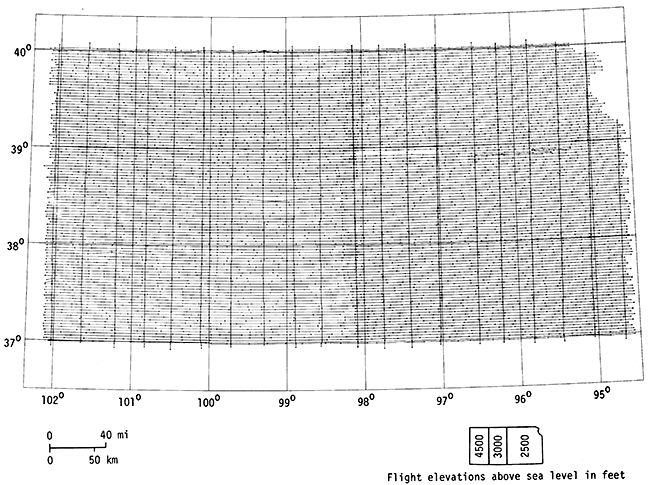
The survey was conducted in eastern Kansas during the summer of 1975 and summer and fall of 1976 and in western Kansas during the summers of 1977, 1978, and 1979. In both eastern and western Kansas the length of the flight lines and tie lines was approximately 340 km (210 mi.) and 345 km (215 mi.), respectively. The flight lines were spaced 3.2 km (2 mi.) apart and the tie lines were spaced approximately 32 km (20 mi.) apart. In eastern Kansas the airplane was flown at a fixed barometric elevation of 762 m (2500 ft.) above sea level. In western Kansas the flight elevations were 915 m (3000 ft.) above sea level in the eastern portion and 1372 m (4500 ft.) above sea level in the westernmost quarter of the State. U.S. Highway 283, aligned north-south through western Kansas, was used as a visual landmark signal to the pilot to change elevations while flying the east-west flight line. The ground clearance, which averaged 366 m (1200 ft.), was measured by the radar altimeter and recorded on magnetic tape along with magnetic measurements. Navigation was accomplished by visual sighting along section roads. The northernmost flight line is located 1.6 km (1 mi.) north of the Kansas-Nebraska border and the southernmost flight line is located 1.6 km (1 mi.) south of the Kansas-Oklahoma border.
Normally the aircraft crew consists of the pilot, navigator, and equipment operator. As a back-up to the flight-path camera, the navigator recorded the time the plane passed over predesignated checkpoints spaced every 15 to 30 km (10-20 mi.) along the flight line. During flight a 24 BCD (binary coded decimal) character record was digitally recorded on magnetic tape with a 7-track, 556 bits/inch tape drive.
To avoid excessive magnetic fluctuation from solar wind disturbance, the magnetic activity k index (Lincoln, 1967) reported from the World Data Center A (National Oceanic and Atmospheric Administration) in Boulder, Colorado, was required to be ~3 before flight takeoff. For k = 4 or 5, the magnetic field was monitored on the ground for at least one half hour before takeoff. If the difference between successive magnetic measurements (noise) did not exceed ±1 nT, the flight proceeded. For k > 6, the flight was cancelled.
After each flight, all records on the magnetic tape were edited for obvious errors such as unreasonable magnetic field values and incorrect bit configurations. The original unedited data were saved on a permanent summary tape. The flight-path film was used to identify landmarks 15 to 25 km (10-15 mi.) apart on 1:125,000-scale county road maps. The longitude and latitude coordinates of landmarks (fiducial points) were digitized on a ±0.025 mm (±0.001 inch) x, y digitizing table and saved on digital tape. The digitizing uncertainty corresponds to ±3.2 m (±10.4 ft.) on the ground. The fiducial-coordinates tape was then merged with the magnetic-field tape for final assignment of longitude and latitude to all magnetic measurements. The resulting flight-path map is presented in Figure 1.
The International Geomagnetic Reference Field 1975 (IGRF) was computed at each measurement location at the appropriate day and subtracted from the total-intensity-magnetic field. These computations were done using the U.S. Coast and Geodetic Survey computer program 609.
The temporal variations in the magnetic field were removed by analysis of the mismatches of magnetic-field values at the tie line-flight line intersections. This procedure, which does not require a recording base station, assumes that diurnal drift during flight is a smoothly varying, low-order polynomial in time. The polynomial coefficients were determined by minimizing magnetic-field residuals at flight line-tie line intersections (for further detail, see Yarger and others, 1978b). Before least-squares adjustment, the intersection residuals were "corrected" by searching for the minimum intersection residual within a 150 m (500 ft.) radius (the estimated uncertainty in the flight-path mapping procedure) of the originally mapped intersection location. After fifth-order temporal variation adjustment to tie lines and flight lines, the residuals were normally distributed about zero with root-mean-square of approximately 3 nT. This residual distribution is adequately narrow to permit contouring at intervals of 5 nT and greater.
Figure 1--Flight paths for aeromagnetic map of Kansas.
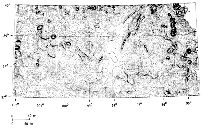
A master grid of total-intensity-magnetic-field values for the State was prepared with 0.16 km (0.1 mi.) east-west spacing and 3.2 km (2 mi.) north-south spacing, which is nearly equivalent to the original measurement spacing. The grid was determined by shifting magnetic-field values from nearly straight flight lines to nearby grid lines. The overall grid location was determined by minimizing (in the least-squares sense) the difference between gridline and the flight-line coordinates. This gridding procedure, which takes advantage of a regularly spaced grid-like flight-line pattern, avoids smoothing that normally occurs when gridded by the available computer algorithms written primarily for arbitrarily spaced data. The master grid, which represents the residual total-intensity-magnetic field, is useful for machine contouring over a wide range of scales and contouring intervals. It is also useful for most quantitative analyses, because the gridding procedure has preserved the original integrity of the data. Figure 2 presents a photo-reduction of the aeromagnetic map contoured by a Kansas Geological Survey computer contouring program at an original scale of 1:500,000 and contour interval of 50 nT.
Figure 2--Aeromagnetic contour map of Kansas. Contour Interval is 50 gammas.
Several spectrally filtered versions of the original contour map (Fig. 2) are used in this regional interpretation. The purpose of filtering a map is to remove certain unwanted characteristics and to enhance desirable characteristics, depending on the interpretation objective. Because of the simple mathematical form of most potential field filters in the spectral domain, it is advisable to transform the original unfiltered map to the spectral domain, apply the filters, then transform the filtered map back to the spatial domain for use in interpretation (Gunn, 1975). A suite of spectrally filtered magnetic maps has proven useful in this study of Kansas basement composition, paleotectonics, and age terranes. Certain filtered maps reveal magnetic patterns, not readily apparent in the original unfiltered map, that are related to basement geology.
An ordinary contour map, where the contoured variable is a function of spatial coordinates, is said to be in the spatial domain. In Figure 2 the contoured variable M(x,y), which is the magnitude of the magnetic field, is a function of the spatial coordinates x,y. The units of x,y are in kilometers (or miles). The map, M(x,y), in the spatial domain was transformed to a map, M(u,v), in the spectral domain using the Fast Fourier Transform (FFT) algorithm (Singleton, 1969) where u,v are the orthogonal spectral domain coordinates. The units of u,v are in cycles/kilometer (or cycles/mile). After applying various filter combinations to the map, M(u,v), in the spectral domain, the resulting filtered maps were transformed back to the spatial domain. "Cycles/kilometer" refers to the number of magnetic highs or lows per kilometer. The characteristic frequency, (u2+v2 )1/2, of a positive (or negative) anomaly is the inverse of twice the anomaly width. For example, an anomaly one-half kilometer wide has a characteristic frequency of one cycle/kilometer. (For further discussion of spectral filtering, see Nettleton, 1976).
Kansas was divided into two equal 216 by 216 grids for input to the FFT program. The grid cell size is approximately 1.6 km (1 mi.) on a side. The eastern and western grids overlapped by 15 cells. The filtered maps were compiled using a variable black-and-white density scale instead of the more traditional contour lines. This format was chosen for several reasons. Density maps are considerably cheaper and faster to produce. Some of the filtered maps have a large dynamic range (i.e., the data range from very large to very small numbers) or may have sharp gradients that are difficult to contour. Finally, the reader can more easily see relative magnitudes on density maps.
Figures 3 through 9 are a suite of seven filtered maps, which are useful in enhancing basement features. These figures are a subset of a much larger suite of filtered maps originally examined. The filtered maps were derived from a combination of two or more filters (see Table 1).
Table 1--Spectral filters applied to Kansas aeromagnetic data.
| Spectral-filter name | Function | Result |
|---|---|---|
| Reduction to the Pole | Removes the effect of the earth's inclined magnetic field. | Improves the resolution and location of anomalies, particularly along north-south direction. |
| Downward Continuation | Recalculates the magnetic field at elevations below flight elevation. | Enhances anomalies caused by near-surface sources. |
| Upward Continuation | Recalculates the magnetic field at elevations above elevation. | Enhances anomalies caused by flight deep-seated sources. |
| High-Frequency Pass | Attenuates low-frequency (long wavelength) signals and passes high-frequency (short wavelength) signals. | Enhances anomalies caused by near-surface sources. |
| Trend Pass | Removes spectral surface trends outside selected directions, passes trends within selected directions. | Enhances anomalies trending in selected directions. |
| Second Vertical Derivative | Calculates second vertical derivative of the magnetic field. | Delineates near-vertical magnetic contacts. |
Figure 3 is a map reduced to the pole and downward continued to 760 m (2500 ft.) above sea level. Reduction to the pole removes the distortion caused by the earth's inclined magnetic field (approximately 650 from the horizontal in Kansas). This results in a slight migration to the north of anomaly maxima and an increase, in some cases, of anomaly amplitudes. All maps appearing in Figures 3 through 9 have been reduced to the pole. The data of the western half of the map were downward continued to 760 m above sea level so as to be comparable to the data of the eastern half, which were recorded at 760 m above sea level. This operation relates all anomaly magnitudes and gradients to the same base level of 760 m above sea level. This is not the case for the original contour map (Fig. 2) in which anomaly magnitudes and gradients are somewhat attenuated in western Kansas relative to eastern Kansas because of the different flight elevations. In the remainder of the text, all maps that have been downward continued to the eastern flight elevation of 760 m above sea level are referred to as "leveled" maps.
Figure 3--Aeromagnetic map reduced to pole and downward continued to 760 m (3500 ft.) above sea level.
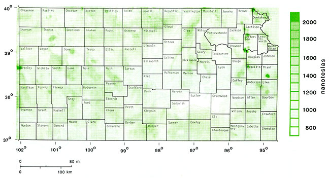
Figure 4 presents an aeromagnetic map upward continued to 9 km (5.5 mi.) above sea level and emphasizes deep-seated, long-wavelength magnetic sources within the crust. Figure 5 presents an aeromagnetic map downward continued to 850 m (2800 ft.) below sea level, which corresponds roughly to the average elevation of the Precambrian surface, and emphasizes magnetic sources at or near the Precambrian surface.
Figure 4--Aeromagnetic map reduced to pole and upward continued to nine kilometers (5.5 mi.) above sea level. The continuous line delineates a possible deep-seated paleoplate boundary within the crust. The dashed lines outline the possible deep-seated boundaries of the CNARS.
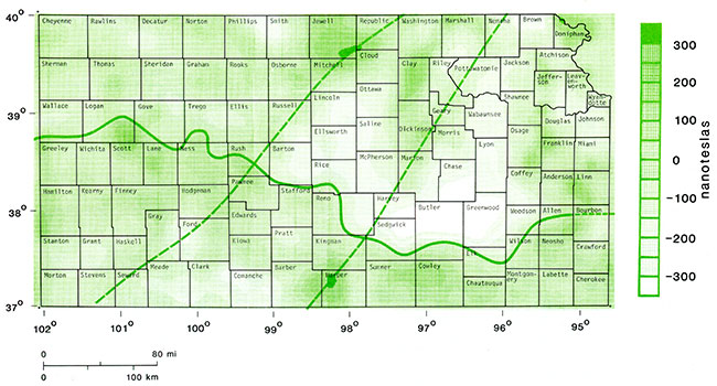
Figure 5--Aeromagnetic map reduced to pole and downward continued to 850 m (2800 ft.) below sea level.
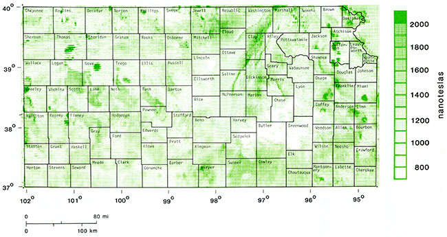
Figure 6 presents an aeromagnetic map leveled and high-frequency pass filtered. This filter passed all frequencies above 0.8 cycles/km and attenuated lower frequencies. We used an attenuation function of 1.25 (u2+v2 )1/2, which is linear in radial frequency. This map emphasizes anomalies caused by magnetic sources at or near the Precambrian surface to a greater extent than does the downward-continued map (Fig. 5). Note that negative amplitudes are not displayed in Figure 6. All amplitudes below +5 nT appear as white. This choice was made to enhance several statewide magnetic trends that are evident in the original maps (displaying the full spectrum of negative and positive amplitudes). There were no significant trends with negative amplitudes that are not also apparent in the positive amplitudes. Negative amplitudes in Figures 7 through 9 were suppressed for the same reason.
Figure 6--Aeromagnetic map reduced to pole, leveled, and high-pass filtered. The continuous line delineates a sharp, high-frequency boundary within the crust. Also delineated are shallow Intrusive plutons.
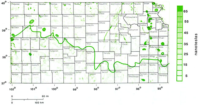
Figure 7 presents an aeromagnetic map leveled, high-pass filtered, and trend-pass filtered. This map is the same as Figure 6 except for the addition of a filter that passes anomalies trending northeast ±45°. This map emphasizes anomalies caused by magnetic sources at or near the Precambrian surface and also trending northeast ±45°.
Figure 7--Aeromagnetic map reduced to pole, leveled, high-pass filtered, and trend-pass filtered northeast ±45°. The continuous lines outline the suggested near-Precambrian surface boundaries of the main part of the CNARS and the southern extent of the Rice Formation.
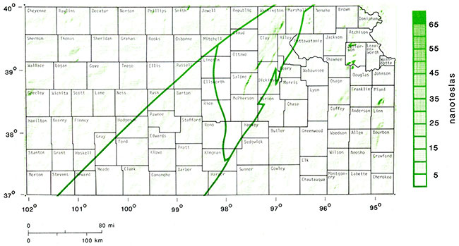
Figure 7, alternative version--Aeromagnetic map reduced to pole, leveled, high-pass filtered, and trend-pass filtered northeast ±45°. The continuous lines outline the suggested near-Precambrian surface boundaries of the main part of the CNARS and the southern extent of the Rice Formation.
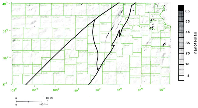
Figure 8 complements Figure 7 and emphasizes anomalies caused by sources at or near the Precambrian surface and trending northwest ±45°. Note that the simple addition of Figure 8 to Figure 7 would yield the original high-pass-filtered map in Figure 6.
Figure 8--Aeromagnetic map reduced to pole, leveled, high-pass filtered, and trend-pass filtered northwest ±45°.
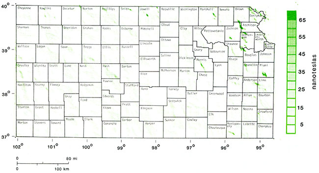
Figure 8, alternative version--Aeromagnetic map reduced to pole, leveled, high-pass filtered, and trend-pass filtered northwest ±45°.
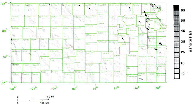
Figure 9 presents the aeromagnetic map leveled, with the second vertical derivative calculated. This map emphasizes near-vertical contacts between contrasting magnetization at or near the Precambrian surface.
Figure 9--Aeromagnetic map reduced to pole, leveled, with second vertical derivative calculated. The continuous lines outline the suggested boundaries of the Keweenawan gabbros and the location of the northern part of the Humboldt fault.
The Precambrian basement complex in Kansas is part of the Midcontinent craton, which is the concealed southern extension of the Canadian Shield. A relatively thin mantle of Phanerozoic sedimentary rocks 150 to 3000 m (500-10,000 ft.) thick covers the basement.
Bickford and others (1981) recently compiled a basement-rock-type map of Kansas and adjacent Midcontinent states, based on available basement-well samples (Fig. 10). The Kansas portion of this map is based on a study of more than 800 thin sections from basement-well samples. The basement terrane in northern Kansas is characterized by granitic to quartz monzonitic intrusive rock, estimated to have been emplaced at depths of 6.5 to 13 km (4-8 mi.). These mesozonal rocks often have cataclastic to extensively sheared textures, particularly along the Nemaha Ridge. Zircon dates (U/Pb) in northeastern Kansas and northwestern Missouri indicate an age of 1625 m.y. for this terrane. In contrast, basement wells in southern Kansas reveal silicic volcanic rocks and associated shallowly emplaced granite. These volcanic and epizonal rocks are not cataclastically deformed and have a nominal age of 1400 m.y.
Figure 10--Map of basement rock types. After Bickford and others (1981).
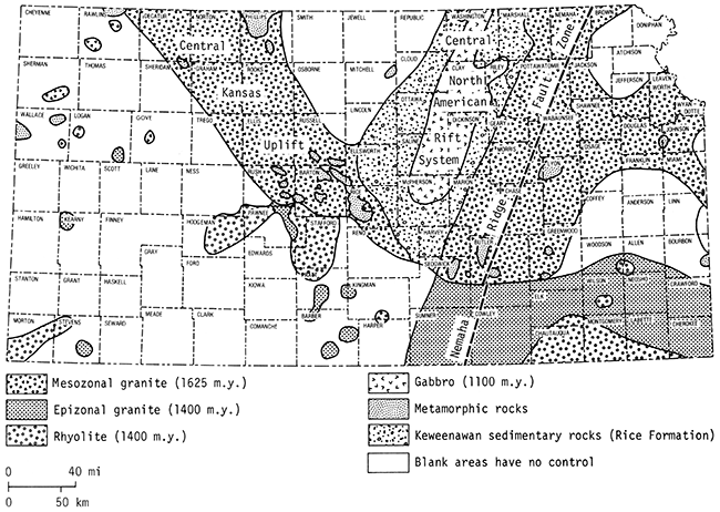
The belt of northeast-trending gabbroic rock in north-central Kansas is the southern extension of the Central North American Rift System (CNARS) (Ocola and Meyer, 1973). This aborted rift system can be traced to the Lake Superior region, where the outcropping rocks are of Keweenawan Age (about 1100 m.y.). A basin of arkosic sandstone to siltstone, designated Rice Formation ( Scott, 1966) in Kansas, flanks and extends to the south of the trough of mafic rift intrusives.
The present structural framework, as depicted in Figures 11 and 12, was formed largely during the late Paleozoic Era and has not materially changed since then. The Nemaha Ridge is a major linear feature, which crosses eastern Kansas from Nemaha County to Sumner County and extends into Nebraska and Oklahoma. The Nemaha Ridge is faulted along the eastern side, where the crystalline basement rocks on the west side of the Humboldt fault are upthrown more than 800 m (2600 ft.) in some areas. The configuration of the Precambrian surface (Fig. 11) exhibits a northeasterly trending grain in a swath through Kansas approximately 145 km (90 mi.) wide and bounded on the east by the Humboldt fault. Outside this zone, the prevailing grain trends northwest.
Figure 11--Configuration of the top of Precambrian rocks in Kansas. After Cole (1976).
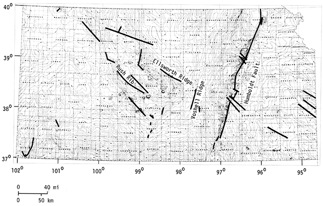
Figure 12--Generalized structural map of the Precambrian. After Merriam (1963).
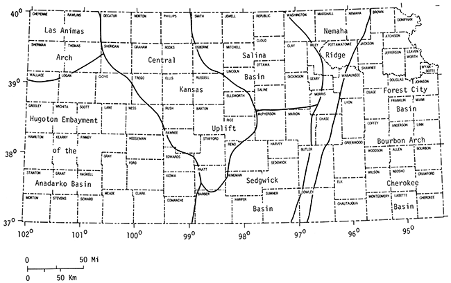
The Forest City Basin is located mostly in Iowa, Missouri, and Nebraska. The southwestern corner, which is the deepest part of the basin, lies in northeastern Kansas and is bounded on the west by the Nemaha Ridge. The Cherokee Basin in southeastern Kansas and northeastern Oklahoma could be considered a shallow southern extension of the Forest City Basin. However, a mildly positive feature, the Bourbon Arch, separates the two basins.
The southern end of the Salina Basin, its deepest part, lies in north-central Kansas. In Kansas it is bounded on the east by the Nemaha Ridge and on the west by the central Kansas uplift. It terminates to the south at an unnamed saddle. Before post-Mississippian deformation, it formed part of the larger ancestral North Kansas Basin. The maximum thickness of sedimentary rocks found in the basin is 1400 m (4600 ft.) (Merriam, 1963). To the south lies the Sedgwick Basin, which is a northern shelf extension of the large Anadarko Basin in Oklahoma. The Hugoton Embayment, which covers much of western Kansas, is also an extension of the much-deeper Anadarko Basin in Oklahoma.
Major variations in strength of the total magnetic field at or near the land surface are normally a result of lateral change in magnetic susceptibility of underlying basement rock. Overlying sedimentary rocks have relatively low magnetic susceptibilities. Susceptibility is proportional to the amount of magnetite in the rock (Clark, 1966). The amount of magnetite in rock is roughly inversely proportional to silica content. For a given volume and depth of burial of source rocks, mafic rocks such as gabbro and basalt will produce larger magnetic anomalies than silicic rocks such as granite and rhyolite.
The relative total-intensity magnetic map (Fig. 2) depicts a rather complex crustal magnetization pattern in eastern Kansas. The dynamic range of the total magnetic field is almost 2000 nT. The contour levels range from 450 to 2350 nT, with an average value of approximately 1200 nT. The base level of the map was established arbitrarily by adding 1500 nT after subtraction of the IGRF from the absolute total intensity. Relative to the IGRF, the magnetic field in Kansas is anomalously low by some 300 nT. If the IGRF accurately describes the large-scale magnetic field intensity in the Midcontinent, then the net magnetization of the crust in Kansas is slightly below average.
Comparison of the magnetic patterns (Figs. 2, 3) with the Precambrian relief map (Fig. 11) reveals little obvious correlation. The Humboldt fault, which has over 800 m (2600 ft.) of vertical displacement in some places, is only weakly discernible. The correlation can be seen in the alignment of magnetic contours along the fault, as in southern Nemaha, northern Pottawatomie, and Wabaunsee counties. The influence of the vertical displacement can also be seen in southern Morris County where the fault trace splits the north-northwest-trending anomaly. The horizontal gradient of the anomaly on the high side (west side) of the fault is steeper than the gradient on the low side. Thus, the source rock for the anomaly was probably emplaced before vertical displacement along the fault. The presence of this anomaly across the fault also suggests no major (less than 500 meters) strike-slip movement along the fault. The difference of 50 nT on either side of the Humboldt fault, which represents maximum basement relief in Kansas, suggests that most other basement relief features in Kansas will have less than a 50 nT influence on the total magnetic field. This is normally the case in areas where the crystalline basement has a fairly thick sediment cover (see, for example, Steenland, 1965). Most of the observed field is caused by intrabasement rock lying below the Precambrian surface and above the depth corresponding to the Curie point isotherm, which is normally 30 to 40 km (19-25 mi.) below sea level. Suprabasement features such as relief and thin lenses of crystalline rock at the basement surface contribute only a small part to the observed field. Suprabasement anomalies are characterized by small magnitudes, sharp horizontal gradients, and short wavelengths and are usually superimposed on large intrabasement anomalies with gentle horizontal gradients and longer wavelengths. Although not considered in this report, suprabasement anomalies are often useful for estimating depth to basement (Nettleton, 1976, Chapter 15).
The total-intensity aeromagnetic maps (Figs. 2, 3) exhibit a northwest-trending grain consistent with the Precambrian surface terrane (Fig. 11 ). This grain is interrupted in northeastern Kansas by the Midcontinent Geophysical Anomaly (MGA) , a northeast-trending linear positive anomaly flanked by adjacent linear negative anomalies. (The positive anomaly, caused by CNARS rocks of gabbroic composition, is discussed in the section on the Central North American Rift System.) The MGA appears to terminate in central Kansas against a roughly linear trend of negative anomalies. This negative trend consists of a nearly continuous band across the State defined by total-intensity amplitude <1200 nT. The most prominent low is centered over Wichita; negative anomalies of lesser magnitude continue westward to the Kansas-Colorado border. This trend can also be traced into Missouri (Missouri Geological Survey, 1943). The southern boundary of this band is clearly visible in the high-frequency-pass filtered map (Fig. 6). This boundary corresponds to a sharp magnetization contrast, suggesting contrasting rock types. This apparent contrast may correspond to a distinct boundary between the older mesozonal granitic terrane to the north and the younger epizonal granitic terrane to the south. This "spectral" boundary is caused by an abrupt attenuation of high-frequency signal, from south to north, and presumably corresponds to the onset of the southern edge of the mesozonal granitic terrane or to some kind of transition zone between the two basement terranes. The northern boundary of the transition zone is not so sharply defined. Outside the CNARS the width of the transition zone varies from 25 to 50 km (15-30 mi.). The zone may correspond to foundered granitic rock overlain by a Precambrian sedimentary or metasedimentary wedge. Alternatively, the band could be caused by nonmagnetic granitic basement. The high-frequency magnetic patterns (Fig. 6) outside of the transition zone and outside CNARS appear approximately the same. The second vertical derivative map (Fig. 9) emphasizes near-vertical contacts between contrasting magnetizations. The boundary, which is outlined clearly in the high-frequency-pass-filtered map (Fig. 6), is not as prominent in the second vertical-derivative map. However, certain portions such as the southern edge of the Wichita low and areas in western Kansas are enhanced. The boundary also is discernible in the upward-continued map (Fig. 4), which emphasizes the deep-seated magnetic character of the crust.
The extreme northeastern portion of the aeromagnetic map (Figs. 2, 3) shows a series of strong, positive, roughly circular anomalies with diameters of approximately 15 km (9 mi.). Basement cores from two of these anomalies, located in Douglas and Miami counties, yielded U/Pb zircon ages of about 1350 m.y. (Steeples and Bickford, 1981). Although these rocks are more coarse-grained than rocks in the southern terrane, they are clearly epizonal granite and related to them (Bickford and others, 1981 ). The Miami County core contains about two percent magnetite by weight (Steeples and Bickford, 1981), which may account for the positive magnetic anomalies. The close similarity of the circular magnetic anomalies suggests that most, or all, of them probably are caused by intrusive bodies similar to those drilled in Douglas and Miami counties. Thus, the 1625-m.y. terrane in northeastern Kansas and northwestern Missouri may be peppered with isolated, shallow granite plutons, possibly related to the 1400-m.y. granitic terrane to the south, but younger by some 50 m.y. This series of circular magnetic highs, along with similar highs in Missouri (Missouri Geological Survey, 1943), roughly track the boundary of the southern half of the Forest City Basin. These mid-Proterozoic granitic plutons may have been intruded along a zone of weakness that later infuenced the formation of the latePaleozoic Forest City Basin.
At least six major near-circular anomalies occur in western Kansas, five of which are closely associated with the granitic terrane boundary discussed previously. Over the entire State there are at least five circular intrusive bodies just to the north of the terrane boundary (Fig. 6). These could possibly be the remnants of volcanic centers associated with Precambrian plate convergence along this boundary.
The pervasive influence of the Central North American Rift System on the Kansas crust is perhaps best seen in Figure 7. This map, which emphasizes high-frequency northeasterly trending anomalies, indicates that the rift system extends south across the entire State.
A magnetic quiet zone, the predominantly white area in Figure 7, surrounds the magnetic high along the mafic belt and corresponds to a basin filled with clastic rocks of (presumably) Keweenawan age. The magnetic quiet zone is caused by the extreme depth to magnetic basement, presumably granite, which foundered during the extensional phase of the CNARS. Both the eastern and western boundaries of this Keweenawan basin are fairly sharply defined, suggesting that they may be fault bounded.
The magnetic lineations to the southwest of the magnetic quiet zone, which are most prominent in Figure 9, probably correspond to block faulting and possibly to mafic dike intrusion that occurred during the initial stage of rifting.
Apparently the rift in southern Kansas did not progress beyond the stage of block faulting and dike intrusion, whereas the rift in northern Kansas developed to a more mature stage of volcanic flows followed by foundered crust and clastic deposits. The fracture system in southern Kansas probably is representative of the crust throughout the CNARS during the early stages of rifting, before upwelling of Keweenawan volcanics occurred. This southwest-trending system indicates that the CNARS extends to the Kansas-Oklahoma border.
The Humboldt fault (Figs. 10, 11), which borders the eastern side of the Nemaha Ridge, closely parallels the CNARS across the State, suggesting that this apparent postMississippian fault may be a reactivated CNARS fault. This Proterozoic forerunner of the Humboldt fault may have developed within the easternmost part of the CNARS crust, which was not involved in subsequent foundering. Alternatively, the Humboldt fault may be a zone of pre-Keweenawan crustal weakness that has been reactivated, or it may not have formed until Paleozoic time.
The trend-pass-filtered maps (Figs. 7, 8) reveal significant magnetic lineations in both the northeast and northwest directions. The most prominent northeast linear trends correspond to the rift system through central Kansas, but a number of northwest trends lie outside the rift, particularly in northwestern Kansas. Figure 8 exhibits northwest-trending magnetic lineations extending over large parts of the state, most of which are interrupted wi thin the rift zone. This, of course, implies that the northwest grain is older than the rift.
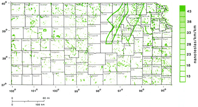
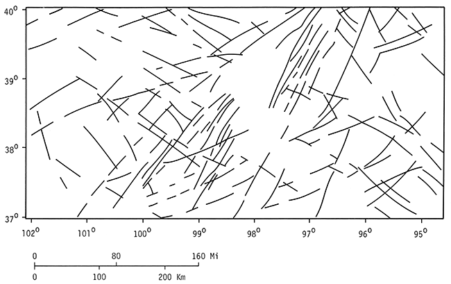
For comparison with known basement structure (Fig. 11), the magnetic lineations apparent in Figures 7, 8, and 9 have been compiled in Figure 13. Determining what constitutes a magnetic linear trend is very subjective. The lineations shown in Figure 13 probably represent "middleground." Other researchers, depending on their criteria and biases, could easily identify more or fewer lineations from the same maps. The lineations we have chosen are at least 50 km (31 mi.) long or belong to a trend of shorter segments at least 50 km long. In addition to suites of northeast- and northwest-trending lineations across the State (seen in Fig. 13), a third suite of east-northeast lineations is evident in southern Kansas.
Figure 13 reveals that the number of magnetic lineations far outnumbers the previously mapped faults (Fig. 11) in the Precambrian. However, a number of one-to-one correlations are evident. The northern half of the Humboldt fault, which borders the eastern sides of the Nemaha Ridge, shows up clearly as a continuous magnetic lineation. The northwest-trending magnetic lineation in Rush County matches the southwest-bounding fault of the Rush Rib. This fault (Merriam, 1963) lies along the postulated Precambrian age boundary (Fig. 6) discussed earlier. Good correlation with the northeast-trending fault segments in western Reno and Pratt counties also exists. The fault through Ellsworth County, which trends northwest along the southwest side of the Ellsworth Anticline, apparently serves as the northern boundary for several of the southwest-trending magnetic linears within the rift zone.
Figure 13--Magnetic lineations. The lineations were derived from Figures 2 and 5 through 9.
The northwest-trending fault in Pawnee County coincides with a magnetic trend that continues to the northwest into Rush County. Part of the southwest-trending fault bounding the northwest side of the Voshell Anticline coincides with a short magnetic lineation at the intersection of McPherson, Reno, and Harvey counties.
Although the northwest-trending magnetic grain in eastern Kansas parallels the Precambrian surface grain, little one-to-one correlation with mapped faults exists. One exception is the fault through Bourbon and Linn counties, which coincides with a magnetic trend that continues northwest into Anderson and Osage counties.
Whether all magnetic lineations correspond to basement faults is an open question. The trend-pass filter operation (Figs. 7, 8) tends to emphasize lineations by elongating them beyond their actual geographical limit. That some of them correspond to known faults strongly implies that at least some of the remaining lineations must also correspond to faults (so far undetected by boreholes). The northeast-trending magnetic lineations within the rift zone must surely correspond to faulting in Keweenawan time. The post-Mississippian movement along the Humboldt fault is most likely a reactivation of a Keweenawan rift fault.
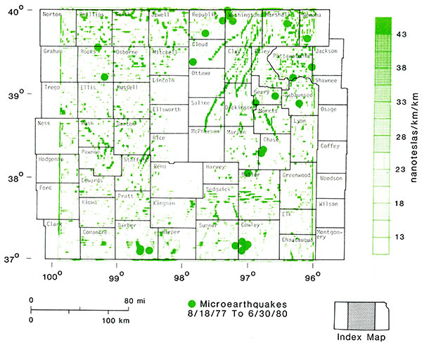
Microearthquake results for the last four years (Steeples, 1980) indicate that the Humboldt fault is still active. The northeastern magnetic trend through Washington, Republic, and Cloud counties, which corresponds to the postulated boundary between the rift sedimentary rocks (Rice Formation) and the older granitic terrane, is seismically active (Fig. 14). Slight evidence (two events) indicates that the eastern boundary between the rift sedimentary rocks and granitic terrane is also seismically active. The only other significant recent seismic activity recorded within the State is located in Barber County and may be related to the southwest magnetic trend through Harper and Barber counties.
Figure 14--Microearthquakes In central Kansas. After Steeples (1980). Microearthquakes are superimposed on the central part of Figure 9.
The recently compiled aeromagnetic map of Kansas (Yarger and others, 1981) is very useful in studying the composition and paleotectonics of the Precambrian crust. Examination of the magnitudes and gradients of the total-intensity-magnetic-field map and of a suite of spectrally filtered maps, in light of existing geologic information, has yielded the following regional interpretation of the Precambrian crust in Kansas.
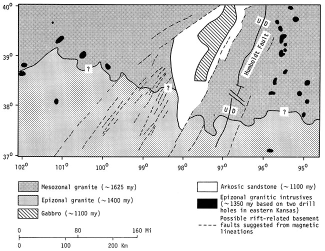
The postulated Precambrian terranes are summarized in Figure 15. A rather distinct boundary appears to exist between the northern 1625-m.y.old mesozonal granitic terrane and the southern 1400-m.y.-old epizonal granitic and rhyolitic terrane, whose magnetic signature is a series of nearly contiguous lows trending west across the State. The southern boundary of this band of lows is sharply defined by steep horizontal gradients and short wavelengths. The magnetic source of this band is not clear. Gravity measurements in this region are being taken by the Kansas Geological Survey; along with potential field modeling, these measurements should help to clarify the origin of this magnetic minimum.
Figure 15--Precambrian terranes in Kansas. Interred from magnetic data and age data of Bickford and others (1981).
Drilling results from two of the 14 circular magnetic highs in northeastern Kansas suggest that the older 1625-m.y.-old crust in northeastern Kansas is pockmarked with younger, 1350-m.y.-old granitic plutons similar in composition to the southern, 1400-m.y.-old terrane of epizonal granite and rhyolite. One to two percent (by weight) magnetite found in the two basement cores may account for the positive magnetic anomalies, whose magnitudes range from 500 to more than 1000 nT.
The CNARS extends through Kansas and probably into Oklahoma. Although large volumes of mafic volcanics clearly did not reach the Proterozoic surface in southern Kansas, magnetic evidence strongly indicates that block faulting and possibly dike intrusion accompanied the initial stages of continental rifting. The southern portion of the 1100-m.y. rift that extends into the 1400-m.y.old crust in Kansas did not evolve into the more mature stages of deep rift-valley formation accompanied by voluminous volcanics and clastics as did the main part of the rift to the north.
Three main suites of magnetic lineations of basement origin are present. Predominately northwest-trending lineations are found in southeastern and northwestern Kansas, whereas central Kansas is dominated by north-northeast-trending lineations. Both of these trends are present in south-central Kansas, resulting in a system of roughly orthogonal intersecting lineations. A third suite of east-northeast-trending lineations is present in southern Kansas. Several of the magnetic lineations correspond to previously mapped basement faults, suggesting that at least a small fraction of the remaining lineations correspond to previously unknown faults. These remaining lineations must be examined by other geophysical methods to establish which ones are faults.
The Humboldt fault, bounding the eastern side of the Nemaha Ridge, parallels the CNARS system, suggesting that it may have developed in Keweenawan time and been reactivated in late Paleozoic time. Recent microearthquake results in Kansas indicate that the Humboldt fault is still active. Some activity along two other magnetic lineations within the CNARS has occurred.
The following University of Kansas students contributed significantly to the aeromagnetic project. Roubik Avanessians assisted in the equipment acquisition, installation, and testing. Robert Robertson's competence was a key influence in all phases of the project, including data acquisition, reduction, and interpretation. Robert Wentland developed several excellent computer programs, including the FFT filtering program. Michael Wolf made some important modifications to the equipment. King Ng did an outstanding job of merging the preliminary partial maps into a final composite data set. James Martin played a key role in data acquisition and reduction during the second half of the project. Rita Sooby efficiently carried out large data reduction and interpretation responsibilities.
We are in great debt to Dennis Sooby, University of Kansas pilot, who devoted a great deal of his personal time to expert piloting of our aircraft. Stewart Giesick, a veteran Beech D-18 pilot, did a commendable job of flying in western Kansas.
I thank William Hinze, Professor of Geophysics at Purdue University, and Lyle McGinnis, Professor of Geophysics at Northern Illinois University, for their thorough review of this manuscript. I also thank Lynn Watney, Don Steeples, and Frank Wilson of the Kansas Geological Survey for their careful review.
This work was supported principally by the Kansas Geological Survey, and in part by special appropriation of the Kansas Legislature for an Automated Resource Evaluation System; by the U. S. Geological Survey, under grant 14-08-0001-G-137; by the U.S. Nuclear Regulatory Commission, under contract AT(49-24)-0256; and by the U.S. Department of Energy, under grant DE-AS07-19ET27204.
Bickford, M. E., Harrower, K. L., Nussbaum, R. L., Thomas, J. J., Nelson, B. K., and Hoppe, W. J., 1981, Rb-Sr and U-Pb and geochronology and distribution of rock types in the Precambrian basement of Missouri and Kansas: Geological Society of America Bulletin, Part 1, v. 92, p. 323- 341.
Clark, S. P., ed., 1966, Handbook of physical constants: Geological Society of America Memoir 97, p. 548.
Cole, V. B., 1976, Configuration of the top of Precambrian rocks in Kansas: Kansas Geological Survey Map M-7. [available online]
Gunn, P. J., 1975, Linear transformation of gravity and magnetic fields: Geophysical Prospecting, v. 23, p. 300-312.
Hinze, W. J. (Chairman), 1976, National magnetic anomaly map: Report of the National Magnetic Anomaly Map Workshop, Golden, Colorado, February 17-19, 1976, 38 p.
Lincoln, J. V., 1967, Geomagnetic indices; in, Physics of geomagnetic phenomena, S. Matsushita and W. H. Campbell, ed.: New York and London, Academic Press, p , 67-100.
Merriam, D. F., 1963, The geologic history of Kansas: Kansas Geological Survey Bulletin 162, 317 p. [available online]
Missouri Geological Survey, 1943, Magnetic map of Missouri: Missouri Geological Survey, scale 1:500,000 (reprinted 1958).
Nettleton, L. L., 1976, Gravity and magnetics in oil prospecting: New York, McGraw-Hill, 464 p.
Ocola, L. C. and Meyer, R. P., 1973, Central North American Rift System 1, structure of the axial zone from seismic and gravimetric data: Journal of Geophysical Research, v. 78, no. 23, p. 5173- 5194.
Robertson, R. R., Yarger, H. L., and Wentland, R. L., 1978, Aeromagnetic map of eastern Kansas (abs.): Kansas Academy of Science Annual Meeting, 110th, Lawrence, Kansas, April 14-15, 1978, Abstracts of contributed papers, Abstract no. 51.
Scott, R. W., 1966, New Precambrian(?) formation in Kansas: American Association of Petroleum Geologists Bulletin, v. 50, p. 380-384.
Singleton, R. C., 1969, An algorithm for computing the mixed radix fast Fourier transform: Institute of Electrical and Electronics Engineers Transactions on Audio and Electroacoustics, v. AU-17, no. 2, p. 93-100.
Steenland, N. C., 1965, Oil fields and aeromagnetic anomalies: Geophysics, v. 30, no. 5, p. 706-739.
Steeples, D. W., 1980, Microearthquakes recorded by the Kansas Geological Survey: Kansas Geological Survey Journal, v. 2, no. 3, p , 14.
Steeples, D. W. and Bickford, M. E., 1981, Piggyback drilling in Kansas: An example for the Continental Scientific Drilling Program: Transactions of the American Geophysical Union, v. 62, no. 18, p. 473-476.
Stevenson, D. J., 1981, Models of the earth's core: Science, v. 214, no. 4521, p. 611-619.
Yarger, H. L., 1979, Spectral analysis of aeromagnetic map of eastern Kansas (abs.): Kansas Academy of Science Annual Meeting, 111th, Wichita, Kansas, March 30, 1979, Abstracts of contributed papers, Abstract no. 36.
Yarger, H. L., 1980, Aeromagnetic analysis of the Keweenawan rift in Kansas (abs.): Transactions of the American Geophysical Union, v. 61, no. 48, p. 1192.
Yarger, H. L., 1981, Aeromagnetic survey of Kansas: Transactions of the American Geophysical Union, v. 62, no. 17, p. 173-178.
Yarger, H. L., Robertson, R. R., and Wentland, R. L., 1976a, Mapping the earth's magnetic field in Kansas (abs.): Kansas Academy of Science Annual Meeting, 108th, Emporia, Kansas, April 19, 1976, Abstracts of contributed papers.
Yarger, H. L., Robertson, R., Wentland, R., and Zietz, I., 1976b, Recent aeromagnetic and gravity data in northeastern Kansas (abs.): Transactions of the American Geophysical Union, v. 57, no. 10, p. 752.
Yarger, H. L., Robertson, R. R., and Wentland, R. L., 1977, The Midcontinent geophysical anomaly (abs.): Kansas Academy of Science Annual Meeting, 109th, Hays, Kansas, April 14, 1977, Abstracts of contributed papers.
Yarger, H. L., Robertson, R. R., and Wentland, R. L., 1978a, Aeromagnetic anomalies in eastern Kansas (abs.): Presented at American Geophysical Union Midwest Meeting, St. Louis University, St. Louis, Missouri, Meeting program and abstracts (AGU Document E79-002).
Yarger, H. L., Robertson, R. R., and Wentland, R. L., 1978b, Diurnal drift removal from aeromagnetic data using least squares: Geophysics, v. 46, no. 6, p. 1148-1156.
Kansas Geological Survey, Regional Interpretation of Kansas Aeromagnetic Data
Placed on web Oct. 11, 2016; originally published in 1983.
Comments to webadmin@kgs.ku.edu
The URL for this page is http://www.kgs.ku.edu/Publications/Bulletins/Geop1/index.html