![]()
Prev Page--The Gamma Ray Log || Next Page--Log Overlay Lithology
Nuclear Logging
The gamma ray log was the first nuclear measurement to be made in boreholes and recorded gamma ray particles emitted from the decay of uranium, thorium, and potassium-40 isotopes. It is characterized as a "passive" nuclear measurement, as contrasted with "active" nuclear measurements that record the response of borehole formations to bombardment by radioactive particles from nuclear sources mounted on the logging tool.
The two most common active nuclear logs are:
- the density log that is made with a gamma-ray source
- and the neutron log that is made with a neutron source
The Density Tool
The density tool typically consists of a radioactive source of gamma rays (e.g., Cesium 137) which is mounted on a rubber pad that is pressed against the formation by the tool.
These constant energy gamma rays radiate into the formation and interact with the electron clouds of the atoms they encounter by Compton scattering, photoelectric effect and pair production processes. As a consequence, there is a reduction in the gamma ray flux which is measured by a short-spaced and a long-spaced detector.
The reason for the two-detector system is to allow for corrections for density perturbations caused by borehole wall rugosity. By combining the two measurements, the density effect of fluid or mud in the borehole wall irregularities can be eliminated. The result is a compensated density log (FDC). The amount of compensation is recorded on the density log as an additional quality control curve. Some zones may be so badly washed out that the density measurement is compromised to the point of being useless. Typically, washout zones occur in thin friable shales.
The reduction in gamma-ray flux is proportional to the average electron density of the formation. The electron density measurements may be converted to apparent bulk density through considerations of a simple atomic theory. The density curve is scaled in units of grams per cubic centimeter and is referred to as the bulk density.
Conversion of Electron Density to Mass Density
Each element can be characterized by an atomic structure of a nucleus comprised of protons and neutrons surrounded by concentric shells of electrons.
The atomic number Z, is the number of protons in the nucleus and is characteristic of the element. This number is equivalent to the number of electrons surrounding the nucleus.
The mass of the atom is contained in the nucleus and is effectively the sum of the number of protons and neutrons. This number is characterized by the atomic mass number, A, which will vary slightly for different isotopes of the same element, in accordance with the varying number of neutrons in the nucleus.
As a general rule, the number of protons closely matches the number of neutrons, with the result that the Z/A ratio of most elements is close to 0.5. This is especially true for elements which are in the lower part of the periodic table, and it is these elements which occur in any appreciable abundance in nature.
Now, since the number of electrons matches the number of protons, electron densities measured by the density tool may be translated to an apparent bulk density in grams per cubic centimeter, by using a Z/A ratio of 0.5.
In logging typical sedimentary lithologies, the difference between apparent and real densities is trivial, since the real Z/A ratios for:
- quartz is 0.4993,
- calcite is 0.4996
- and dolomite is 0.4994.
However, there is a measurable difference for some commonly encountered minerals, for which halite provides the best example. The density log apparent density for halite is 2.03 while its real density is 2.16, owing to its actual Z/A ratio of 0.4799. These differences are of little concern in log analysis, as calculations are made consistently in terms of apparent density. However, errors may be introduced by the use of real densities, unless they have been modified to their apparent equivalents through correction by a Z/A factor appropriate to their atomic composition.
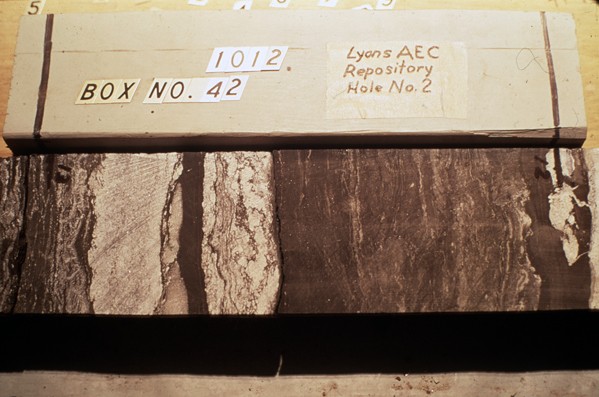
Example of a Density Log in an Evaporite Sequence
The U.S. Atomic Energy Commission test hole AEC #2 was drilled in Rice County, Kansas in 1970 to evaluate the potential of the Permian Hutchinson Salt as a storage facility for low-level radioactive waste. The hole was continuously cored through the Wellington Formation and logged with a full suite, including a density log.
The illustration shows a section at the base of the Hutchinson Salt, which overlies interbedded anhydrites and shales. The lithologies are marked in the depth track, as transcribed from the core description.
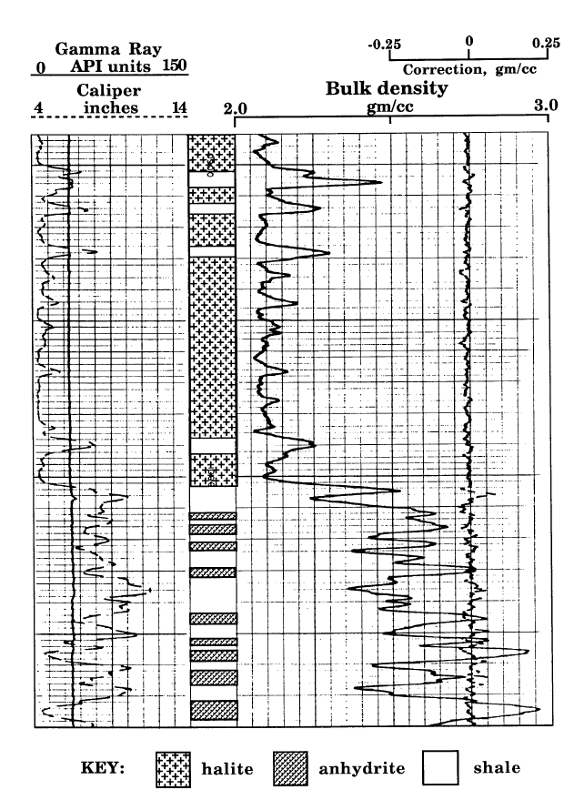
The well was drilled with salt-saturated mud, so that the caliper in Track 1 shows a fairly constant borehole diameter that matches the bit size.
The gamma-ray curve in Track 1 show very low values for the halite of the Hutchinson Salt, interspersed with some shaly layers. Below the salt, the gamma-ray fluctuates between shale and anhydrite beds.
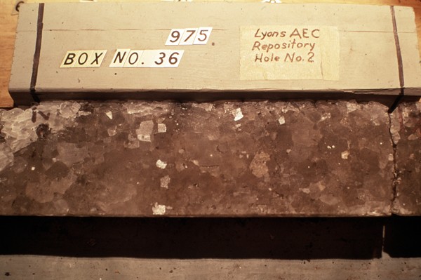
Halite at 975 feet depth
Anhydrite and shale at depth of 1012 feet
On this log presentation, Tracks 2 and 3 are combined. The bulk density curve is scaled conventionally between 2 and 3 grams per cubic centimeter. This range accommodates most sedimentary lithologies. In the event of a zone with a density that is less than 2 gm/cc (such as a coal bed), the curve would be shown on an additional secondary scale of 1 to 2 gm/cc. Similarly, the density curve for zones with densities greater than 3 gm/cc would be displayed on a supplementary scale of 3 to 4 gm/cc.
As mentioned previously page, the expected log density for pure halite is 2.03 gm/cc. The Hutchinson Salt shows slightly higher values of approximately 2.07 gm/cc that reflects small quantities of impurities, which are probably clay material. There is a dramatic contrast with the expected log density for pure anhydrite, which is 2.98 gm/cc. The bulk densities of some of the lower anhydrite zones almost reach this value, but there is a progressive thinning of anhydrites moving upwards below the vertical resolution of both the gamma-ray and density tools (2 to 3 feet), resulting in some averaging with the interbedded shales.
Unlike specific minerals such as halite and anhydrite, the density of shales is highly variable in sedimentary successions as determined by degree of compaction, proportion of clay minerals, and density of non-clay components. So, the density of a shale is read directly from the density log.
Porosity from the Density Log
Although the density log was originally introduced to calibrate gravimetric surveys by geophysicists, its application to porosity measurement was quickly realized. Consequently, it is common practice to see a density log presented both as a curve scaled to bulk density in grams per cubic centimeter and scaled to pore volume.
The conversion of bulk density to porosity uses a simple mass balance relationship, by interpolating between the matrix mineral density in grams per cubic centimeter:
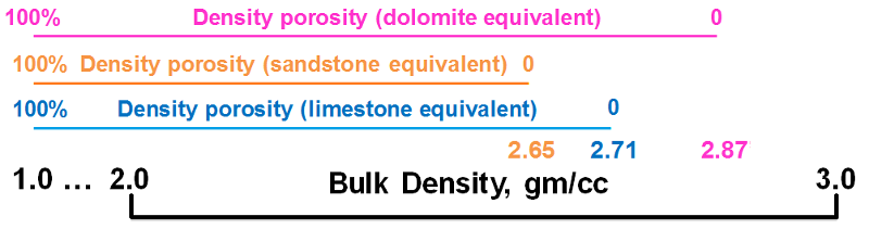
- 2.65 quartz
- 2.71 calcite
- 2.87 dolomite
and mud filtrate, with a density of 1.00 gm/cc for fresh mud.
These endpoints correspond to the three major reservoir lithologies of sandstone (quartz), limestone (calcite), and dolomite (dolomite).
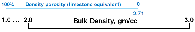
1.When calibrated to the bulk density, the limestone scale porosity would look like:
Limestone-equivalent porosity scale
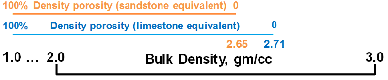
2. If we added a porosity scaled for sandstone, we would see:
Limestone-equivalent and sandstone-equivalent porosity scales
and 3. finally, if we added a porosity scaled to dolomite, we would see:
Limestone-, Sandstone-, and Dolomite-equivalent porosity scales
The choice of matrix (mineral) to be used for scaling is under the control of the logging engineer.
In target zones of sandstone sedimentary successions, the conventional choice would be a sandstone matrix, computed using a quartz value of 2.65 gm/cc. In a limestone-shale sequence, the choice would be a limestone. The logging engineer's choice is marked on the scale (see example below).
In sequences of multiple lithologies (sandstones, limestones, and dolomites), the limestone scale is commonly used as the default scale. The correction of the apparent limestone porosity to true porosity in other lithologies is then made by incorporating information from the neutron porosity, as will be described later in this lesson.
In the example above, we see a density porosity index scaled in porosity units that is calibrated for a limestone.
The zero value for the porosity index is set to 2.71 gm/cc and the 100% porosity is matched with a mud filtrate density of 1.00 gm/cc.
Two important points are:
- In common with all porosity logs, the porosity is shown increasing towards the left (not a conventional expectation)
- While negative porosity is clearly impossible, the scale is set for an apparent porosity. Any zone with a greater bulk density than a limestone with zero porosity (i.e. calcite, density 2.71 gm/cc) will appear to have "negative porosity."
The Photoelectric Factor (PeF) Log
The photoelectric factor (PeF) was introduced in the early-1980's as a supplementary measurement to the bulk density measurement and records the absorption of low-energy gamma rays by the formation in units of barns per electron.
The logged value is a direct function of the aggregate atomic number (Z) of the elements in the formation, and so is a sensitive indicator of mineralogy. For any given element, the index is given by the formula:
PeF = (Z/10)3.6 *wt
This means that the expected PeF for any mineral can be calculated, given its formula, by summing the separate elemental contributions multiplied by their weight. However, this is not necessary in practice, because the values for a wide range of minerals are tabulated online by logging service companies.
This relationship and the fact that the value is only mildly affected by pore volume magnitude or fluid/gas content, means that the index is an excellent indicator of mineralogy.
Basic mineral reference values for the common sedimentary lithologies of sandstone, dolomite, and limestone are:
- quartz 1.81
- dolomite 3.14
- calcite 5.08 barns/electron.
The photoelectric factor is unable to distinguish between chert and sand because they are both silica with the same aggregate atomic number.
The photoelectric index log is commonly scaled on a range between 0 and 10 barns/electron, and a generalized interpretation guide is given in the figure below.
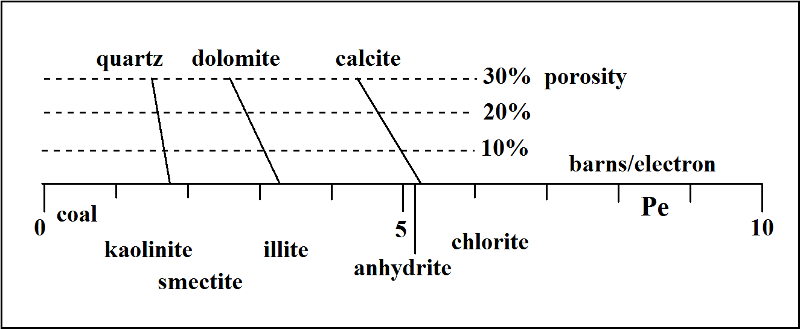
On this scale, minerals such as calcite, dolomite and quartz have narrowly defined expected values, with a minor downward drift at increasing porosities in their host lithologies. Notice that anhydrite and calcite have similar photoelectric factor values. However, anhydrite would be easy to distinguish by looking at the density curve where its expected value of 2.98 would be much higher than limestones which would be less than 2.71 gm/cc.
Although the photoelectric factor curve is controlled by mineralogy, it is routinely used in conjunction with gamma-ray, density and neutron porosity curves in order to resolve ambiguities in interpretation. So, for example, a PeF value of 3 barns/electron could be dolomite, but it could also reflect a mixture of quartz and calcite. The same value could also match an illitic shale and this interpretation could be checked by looking for a shale response on the gamma-ray curve.The collective examination of all these curves for a full geological interpretation will be reviewed in the next lesson.
The compositional variation of clay minerals means that their position on the photoelectric factor scale shown above should only be taken as a broad indication. Based on its aluminosilicate composition, kaolinite has a similar expectation of PeF value to quartz. The ordering of other clay minerals on the index is almost entirely a function of their likely content of iron.
Occasionally, zones will occur with anomalously high photoelectric factor values and these reflect the occurrence of a significant content of an element with a high atomic number. In almost all cases, this signifies the occurrence of some iron-bearing mineral such as pyrite or siderite. The occurrence of these minerals will also be reflected by high bulk densities.
The Neutron Tool
Neutron tools contain a radioactive source that supplies a flux of high energy neutrons that radiate spherically into the rock at the borehole wall. These neutrons lose energy each time that they collide with nuclei of atoms on their travel through the formation.
The greatest loss in energy occurs when neutrons collide with nuclei that have a similar mass. Consequently, collisions with hydrogen atoms account for the major proportion of neutron moderation in most rocks.
The fast neutrons experience a progressive loss in energy, first to an epithermal state and ultimately to a thermal state, at which time they are vulnerable to capture by a nucleus with a high capture cross section. Most commonly, the element that absorbs these slow moving neutrons is chlorine, contained in the salinity of the pore water. In absorbing a neutron, the nucleus emits a gamma ray with a characteristic energy.
Older tools had a single detector and measured either the quantity of capture gamma rays or epithermal neutrons. Modern devices have two detectors of thermal neutrons located at a short distance from the source to compensate for borehole effects. Because the reduction in neutron flux is controlled to such an extent by the formation hydrogen concentration, the measurement can be used for porosity estimation in typical reservoir lithologies.
Porosity from the Neutron Log
At the most fundamental level, a neutron log records the amount of hydrogen in the formation, regardless of whether the hydrogen occurs in a gas, solid, or liquid. However, the commercial application of this measurement is to assess the porosity in potential reservoir zones.
Although the older logs were recorded in neutron counts, almost all modern neutron logs are scaled with respect to porosity. As with all porosity logs, the porosity increases to the left on the scale.
In a similar fashion to density porosity scales, the neutron log is anchored to two calibration points: the matrix and the fluid. The matrix choices are calcite, dolomite, or quartz. These have slightly different neutron moderation characteristics, so that the zero porosity point differs slightly, depending on whether the scale selected is limestone-equivalent, sandstone equivalent, or dolomite equivalent. The logging engineer has control on this decision which may be made to match the predominant lithology of the logged section. For multiple lithology types, the default selection is a limestone scale.
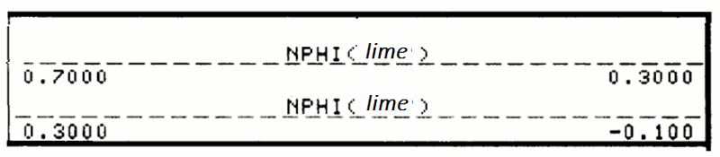
The units can either be in percent (often written as "porosity units" or "p.u.") or in decimal units (zero to one), as in this example. Notice that the logging engineer has indicated that the scale is for limestone-equivalent porosity by the parenthetical "lime".
The primary scale range of -0.1 to 0.3 is a common choice, but the engineer may make a scale change. So, for example, a range of -0.15 to 0.45 might be chosen for sections with high neutron porosities, so as to keep the curve in range, without annoying wrap features. In cases where the neutron porosity exceeds the range of the primary scale, it will be displayed on the secondary scale.
As with the density porosity, negative values do NOT indicate error. Because the porosity scale in this example, is set for limestone, a zero porosity represents the neutron moderation of calcite. So, for example, a sandstone or chert bed with zero porosity, would read slightly negative on a limestone-equivalent neutron porosity scale.
Because the neutron log is actually a response to the hydrogen in the formation, regardless of its presence in a gas, liquid, or solid, hydrogen-rich lithologies will show high neutron porosities, even though there is no effective pore space. Examples include:
- shales--water that is bound to the clay minerals will cause relatively high neutron porosities. The value will depend on the amount of bound water, which is controlled by the degree of compaction. In addition, the hydrogen within the clay aluminosilicates will be a contributory factor.
- water of crystallization--some evaporitic minerals, such as gypsum have water of crystallization. Gypsum is a hydrated form of calcium sulfate with a formula of CaSO4 · 2H2O. The gypsum response exceeds 60% equivalent limestone porosity on a neutron log.
- hydroxyls--minerals that have a hydroxyl component (OH). Goethite is an example, with its formula of FeO(OH), results in a neutron porosity reading in excess of 60%.
- coal--the high neutron porosities of coals are caused by their high moisture content. Their neutron porosity varies by rank so that anthracite has an expected value of about 38%, while bituminous coals have much higher values.
In contrast with these high hydrogen sources, the occurrence of gas is marked by anomalously lower neutron porosities. The neutron porosity scale is calibrated to a pore content of water. Both water and oil have a high concentration of hydrogen per unit volume of pore space. However, hydrogen is relatively diffuse in a gas such as methane, so that the recorded neutron porosity is less than the actual pore volume. Together with the density porosity, which becomes anomalously higher with gas saturation, the "gas effect" has commercial implications in the recognition of gas zones.
Example of a Neutron Log in a Limestone-Shale Sequence
A compensated neutron log is shown in for a Pennsylvanian Kansas City Group "J" zone from a well in southwest Kansas.
The 'J' zone is a thick limestone underlain and overlain by marine shales, which are probably dark and with some uranium content as suggested by their gamma-ray readings of about 180 API units (see Track 1). These shales also have neutron porosity readings of about 34 limestone-equivalent porosity units.
Within the 'J' limestone, low porosity intervals correspond to wackestones which represent open-marine micritic sediments that were deposited on a broad open shelf.
These wackestones are contrasted with a high porosity oolitic grainstone unit that was formed in an oolite shoal.The porosities reach 33% and are caused by the development of oomoldic pores, where ooids have been dissolved to form spherical molds.
Watney (1985) used the high porosity signature of the oolitic facies to map the thickness of this regressive carbonate, and so outline the distribution of oolite shoals on the ancient shelf. Northward-pointing fingers that punctuate a broad facies belt appear to resemble modern spillover lobes of oolite in the Bahamas. Watney (1985) concluded that the "J"-zone oolite distribution indicated the location of a break in the Pennsylvanian shelf paleoslope with a strike approximately west to northwest. This break probably became a focus for waves and currents active in the shoaling conditions within this limestone unit.
Oomodic limestones are units that contain important oil and gas reservoirs, both in Kansas and the Middle East.
True Porosity from the Overlay of Density and Neutron Logs
It is now common practice for logging service companies to run density and neutron measurements on the same tool and present their readings as an overlay.
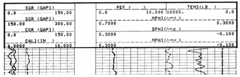
This is shown in the typical example above, which may appear confusing at first but should be approached with a similar frame of mind to that of an aspiring pianist who is confronted by sheet music. In both cases, the paper record has a grid convention to display information and its mastery is a matter of practice, rather than an intellectual puzzle.
Which curve is which? The style of each scale (solid, dashed, dotted) is matched with the style of the curve.
In Track 1 we see both SGR and CGR gamma-ray curves which tells us that a spectral gamma-ray tool was run.The CGR is low, and since it responds to potassium and thorium, suggests that there is little clay content. Consequently, the zone is not a shale, but a potential reservoir zone.
Both the neutron and density porosities were scaled to an apparent limestone equivalent but show markedly different values. Which is correct? They are both wrong! The lithology effect (in this case a dolomite) causes the neutron porosity to read too high and the density porosity to read too low. So, the true porosity, as an estimate of the actual volume of pore space, is somewhere between these two values.
A limestone-equivalent porosity is a good choice for both neutron and density logs, because calcite has properties that are intermediate between dolomite and quartz. By averaging the apparent neutron and density porosities of a zone, effects of dolomite and quartz tend to cancel out. The true porosity may be estimated either by taking an average of the two log readings or a more accurate estimate is made by crossplotting the neutron and density porosities in a service company chartbook.
The estimation of the true volumetric porosity is a matter of eliminating the lithology effects on the neutron and density curves. However, these same lithology effects are the basis for interpretations of mineralogy and lithology, particularly when used in conjunction with the photoelectric factor curve. Because this combination is run routinely in thousands of wells all over the world, the geological interpretation of logs is an everyday skill that moves beyond basic correlation of formation tops. We shall develop this skill in the next few lessons.
Prev Page--The Gamma Ray Log || Next Page--Log Overlay Lithology
Kansas Geological Survey
Updated July 31, 2017.
Comments to webadmin@kgs.ku.edu
The URL for this page is http://www.kgs.ku.edu/Publications/Bulletins/LA/04_nuclear.html