![]()
Prev Page--Contents || Next Page--Digital Logs
The Logging Operation
The First Log
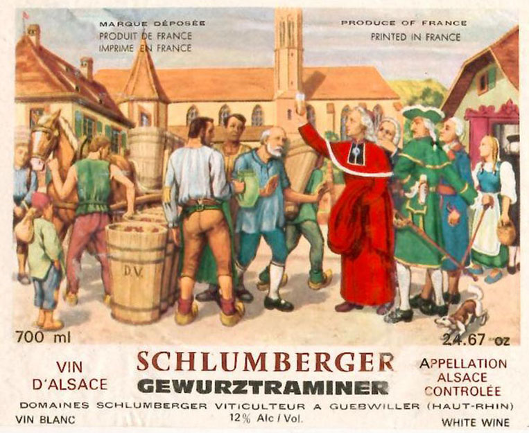
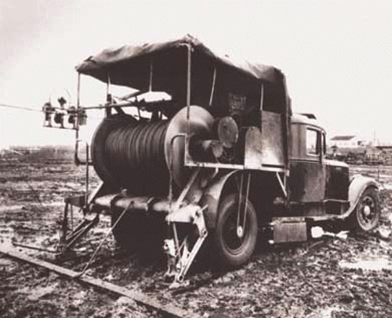
Conrad and Marcel Schlumberger were geophysicists from Alsace-Lorraine in France, where the Schlumberger family were powerful landowners. The brothers originally worked with surface electrical prospecting techniques in the search for ore bodies and petroleum. In 1927, as a result of a conversation with the manager of a Franco-Belgian drilling company, Conrad arranged for his son-in-law, Henri Doll to attempt the first experimental resistivity survey in a well. In the Pechelbronn oilfield in Alsace, the top of the Hydrobiae marls was used as a stratigraphic marker, but was sometimes missed or misidentified in drilling. Consequently, the problem the resistivity survey would attempt to solve was whether the technique could be an effective means to recognize subsurface formations for use in correlation and mapping.
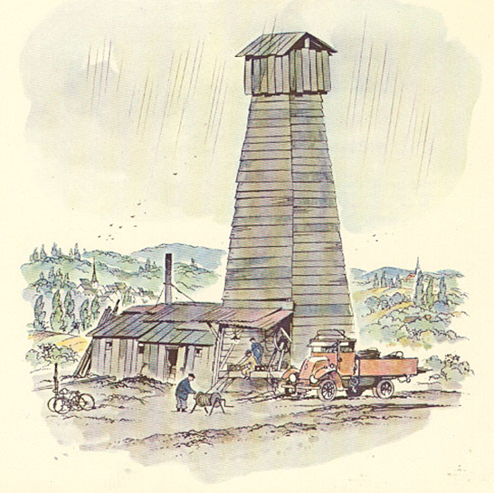
Doll put together a four-electrode (lateral) resistivity device and drove out to the well Diefenbach 2905, Tower 7, together with Scheibli and Jost on September 5, 1927. There, they linked the sonde weighted with lead to three conductive cables spliced together with insulating tape, loaded it onto a hand-operated winch, and attached it to batteries and a potentiometer. The first run was to 140 meters and took 15 hours largely because of interruptions caused by breaks in the cable. A new and longer cable was brought in by taxi to allow them to reach the full well depth of 600 meters. Resistivity readings were taken at one-meter intervals in a slow process that gradually speeded up as they became more practiced.
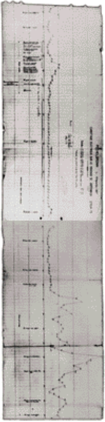
On returning to Paris, Doll plotted the resistivities as a function of depth and, by joining the points, drew the first electric log. Because the well had been cored, the geology was known, so that useful comparisons could be made with the resistivity curve. The Hydrobiae marls were recognized as a zone of uniformly low resistivity which was succeeded by a mixed sequence of conglomerates, sandstones and hard marls. which were distinguished by more resistive peaks and troughs. Logging runs in neighboring wells showed that many of these resistivity features could be recognized and correlated laterally. The new method was called "electrical coring"; the term "electrical logging" did not replace it until 1933. It is interesting to notice that this first log was run for a specific geological purpose--to see if borehole resistivity measurements could be used to recognize lithologies to aid in stratigraphic correlation.
Early Logging in Kansas
The oldest known log in Kansas was recorded on July 16, 1935 by the Schlumberger engineers J.C. Legrand and R.I. Seale for the Shell Oil Company in the Oxford field in Sumner County.
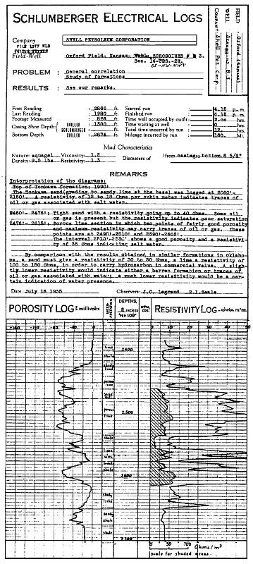
In addition to a resistivity log, a so-called porosity log is also recorded, but its units of millivolts show it to be an SP (spontaneous potential) log. Deflections of the SP ("porosity") log to the left indicated porous and permeable potential reservoir units of either sandstones or limestones, contrasted with shales that plot to the right, The resistivity log contrasted low-resistivity shales with higher resistivity sandstones and limestones.
However, the remarks on the log header demonstrate the rapid advance in understanding of this new technology in the recognition of porous and hydrocarbon-bearing zones in addition to subsurface unit recognition for stratigraphic correlation. Potential reservoir units were evaluated by the engineers and they also summarized the guidelines that they applied in their interpretation as:
"By comparison with the results obtained in similar formations in Oklahoma, a sand must give a resistivity of 30 to 50 Ohms, a lime a resistivity of 100 to 150 Ohms, in order to carry hydrocarbon in commercial value. A slightly lower resistivity would indicate either a barren formation or traces of oil or gas associated with water; a much lower resistivity would be a certain indication of water presence."
Since that time, hundred of thousands of logs have been recorded in wildcats and production wells across Kansas. Although their primary use is for subsurface correlation purposes, log interpretation and analysis has always been a key component of judgements in wildcats and reservoir development of fields. Paper copies of all logs run in Kansas have been filed with the Kansas Corporation Commission (KCC) and made available to the public after a two-year confidentiality period through the Kansas Geological Survey in Lawrence and the Kansas Geological Society in Wichita. Recently, the requirement has been modified to collect electronic files in the form of digits as both LAS files and image files. These electronc log files can be downloaded from the Kansas Geological Survey as a free service. In a lesson activity later in this course, you will be instructed on how to download an LAS file from the KGS website onto your computer and how to open it using standard software.
Fast Forward: Modern Logging Operations
Prior to drilling a well, a logging program is chosen with a suite of tools to be run that is suitable for the target formation petrophysical properties, the engineering characteristics of the hole (mud type, hole diameter, etc.), and the problems to be resolved by the tool measurements. The logging company is chosen for the job.
When the hole approaches the target total depth, the logging company is contacted and a logging truck is sent to the location of the drilling rig. The wireline logging crew typically has a field engineer, who directs the logging, and two equipment operators.
The crew prepares for logging as the drill-pipe is tripped out of the hole. They lay the tool parts out on the catwalk, calibrate them, and assemble them into a tool.
When the drill-pipe has been removed from the hole, the tool is attached to a cable and lowered down the hole.
The length of the tool is variable, but can be anything between 20 and 100 feet (or more).
In the plan for the drilling, some allowance will have been made for the anticipated tool length by drilling an extra depth of "rat-hole", beyond the desired total depth.
Logging a well in southern Kansas
This Schlumberger truck has come from Sugarland, Texas with some specialized logging tools.
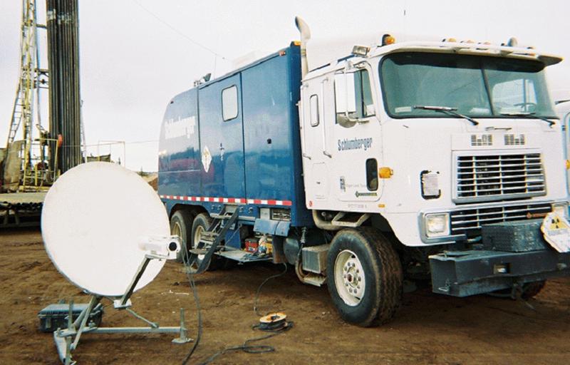
Although Schlumberger is now a major multinational corporation, the truck colors of blue and white reflect the comany's origins in France, as these are the colors of the French national racing team.
The logging truck was constructed in Houston to include expensive and sophisticated logging tools as well as computer systems for telemetry and data aquisition.
Notice the radioactivity sign on the front of the truck that reflects the radioactive sources for neutron and density logging.
The dish at the left transmits the logging measurements to a log analyst at a remote location for immediate evaluation.
A view of the back of the same truck
The winch controls the lowering and raising of the logging tool attached to the logging cable. The cable is the "wireline" of "wireline logging."
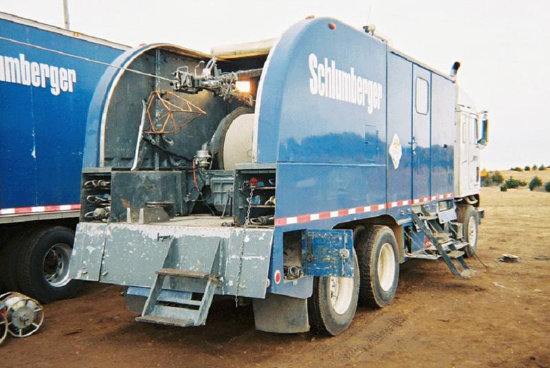
The drums on the ground to the left contain the radioactive sources for neutron and density logging, which are carefully inserted into the tool prior to logging.
The Logging Run
Logs are normally not recorded as the tool is lowered into the hole. Instead, the log measurements are made as the tool is raised from the bottom of the hole, when an even tension on the cable is easier to maintain and so ensure potential good depth registration.
On reaching bottom , the total depth (TD) is measured either from ground level (GL) or the Kelly Bushing (KB) of the drilling platform, and compared with the drill crew's estimate. The total depth estimates may match, although the logging engineer's estimate is often slightly shallower, if the tool was not able to reach the bottom of the hole.
The logging crew is now ready to record logs.
|
|
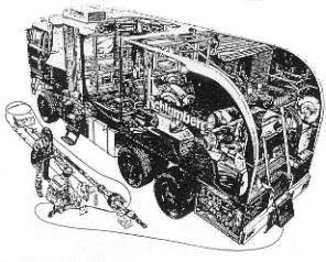
In the cartoon to the left, the tool is at the bottom of the hole. The sensors are located at various positions along the tool, shown symbollically by the yellow circles.When logging is started, the first reading (FR) of each measurement willl start at different depths. This is the reason why an extra length of rat-hole is drilled to ensure that the formation of interest at the bottom of the hole is logged completely. First, the tool is raised through 100 to 200 feet in an initial recording pass, that creates the "repeat section." The tool is lowered back to the bottom and the main run initiated as the tool is pulled through the entire hole. A comparison between the main run and repeat section is made for a quality assurance of repeatability (precision). The field engineer checks this, as does a company representative (the well-site geologist or engineer), who also does other quality checks on the final log. The company person will sign off as the witness if he or she is satisfied; if not satisfied, another run will have to be made. The logging tools are pulled up at a uniform speed so as to maintain a fairly constant tension in the steel cable. The logging speed varies with the type of physical measurement, but is usually between 1800 to 3600 feet per hour. Sometimes, the tool may get stuck in the hole and then (hopefully) spring free, and these problem intervals will show on the tension log and warn that log depths there will have some error. The logging crew will also take a sample of the drilling mud and measure the resistivity of the mud and the mud filtrate in a conductivity cell in the logging truck. These are recorded on the log header. |
The old logging trucks recorded logs in analog form as "blue-lines" that were photographically developed in the truck. Modern logging equipment is computerized, with logs recorded digitally. Both hard-copy blue-lines and digital files can be supplied to the company representative at the well-site. In the case of major company wells in remote locations, the logging information can be bounced off a satellite and analyzed immediately by a petrophysicist in a company office.
The Log Format
At the top of the log is the header which records:
|
|
The bulk of the log contains the curves recorded on the main run:
In the tail of the log is the repeat section--the curves recorded on a short initial run from the bottom of the logged section and used for a quality control check on the main run. |
The log is terminated by calibration data associated with the tests on the tools run in this borehole.
Example: A Wildcat Triple Combo Logging Run
The Bill Barrett Corporation wildcat #12-24 Helman P was drilled as an exploration hole in Sherman County, western Kansas in search of commercial gas production from the Cretaceous Niobrara Chalk. Shallow biogenic gas fields have been developed in the Niobrara of Colorado, Kansas, and Nebraska for many years. The target Niobrara interval for maximum production is known as the "Beecher Island zone."
The header for the triple combo logging run together with the tool conguration is shown below:
In reading the header, we see that the logging run was made on March 23, 2005 and that the well is located in Section 24 of Township 6 South, Range 40 West.
The Start of the Logging Run--First Reading
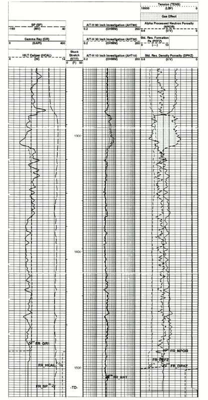
Here are the logging curves recorded at the bottom of the hole:
Track 1: Caliper, gamma-ray, and SP (spontaneous potential) logs.
Track 2: Array induction resistivities
Track 3: Density, neutron, and the photoelectric factor
Notice that each curve can be identified separately by reference to the scale line strengths. So, for example in Track 1, the caliper is dashed, the gamma-ray curve is solid, and the SP is bold-dashed.
The position of total depth (TD) is marked in the depth track. the deepest location of each log curve is marked by FR (First Reading). In each case the "curves" below the FR are meaningless. The relative poisitions of the log curve FR's match the corresponding sensor location on the tool as shown by the configuration on the header.
The Repeat Section
Comparison of the repeat run with the main run:
The overlay comparison of the logging curves recorded in the repeat run (Pass 1) with the bottom of the main run (PASS 2) is part of quality control. If the curves match closely, then it shows good precision, but says nothing about accuracy. The issue of accuracy is addressed by calibration checks that the engineers make prior to logging.
The Main Logging Run
The curves from the main logging run:
Notice the total depth (TD) marked in the depth track and the relative positions of the first reading (FR) for the individual log curves.
The Beecher Island Gas Zone
Let's focus our attention on the Beecher Island Zone towards the top of the logged section, which is marked by a strong gas effect on the neutron and density porosity curves:
Track 1: The "Beecher Island Zone" is located where the gamma-ray curve decreases ( towards the left in Track1). The logging engineer expanded the gamma-ray scale to 400 API units beyond a conventional 150 API unit limit because the Niobrara Chalk is relatively radioactive. The source of this radioactivity is uranium, which is linked with the high kerogen content of the Niobrara. Kerogen is organic matter, whose biogenic alteration is the source of the gas that has accumulated in the Beecher Island Zone.
Track 2: Notice the increase in resistivity in the Beecher Island that reflects the higher resistivity of the gas zone
Track 3: A classic "gas effect" is shown in Track 3 where the density log shows a high apparent density porosity (increasing to the left) because of the low density of the gas, and a low apparent neutron porosity, because of the low concentration of hydrogen atoms in gas. This "crossover" effect between the two curves is highlighted on the log by the dotted pattern. Both the neutron and density porosity curves are scaled for limestone and water. Below the Beecher Island Zone, the neutron porosity curve reads higher than the density (to the left) because the chalk is not a pure limestone, but a marl, whose clay content has bound water. The neutron porosity curve increases (to the left) because of the additional hydrogen introduced by the clay water.
The interpretation remarks above represent a basic reading of the logs and are introduced at this early stage to give an idea of how much information is available on a standard log presentation. As Yogi Berra once said, "It's amazing what you can see, just by looking." As the course develops, you will acquire the interpretation skills to make assessments like these.
This well was perforated in the interval 1281-1313 feet depth with an initial production (IP) of 40 MCF per day. The wildcat Helman P #12-24 resulted in a discovery well for the Prairie Star Field with gas production from the Beecher Island zone of the Niobrara Chalk Formation. The Prairie Star Field was subsequently merged with the Goodland Niobrara Gas Area.
In the next lesson, DIGITAL LOGS, you will gain practical experience in downloading an LAS digital log file from this well onto your computer.
Prev Page--Contents || Next Page--Digital Logs
Kansas Geological Survey
Placed on web March 24, 2017.
Comments to webadmin@kgs.ku.edu
The URL for this page is http://www.kgs.ku.edu/Publications/Bulletins/LA/01_logging.html