Kansas Geological Survey, Open-file Report 94-28b
Part of the Mineral Intrusion Project: Investigation of Salt Contamination of Ground Water in the Eastern Great Bend Prairie Aquifer
A cooperative investigation by The Kansas Geological Survey and Big Bend Groundwater Management District No. 5
KGS Open File Report 94-28b
Released December, 1994
To read this report, you will need the Acrobat PDF Reader, available free from Adobe.
The Mineral Intrusion project has as one of its primary objectives the determination of the amount, distribution and movement of naturally occurring saltwater in the Great Bend Prairie aquifer. Background information on the objectives, setting and methods of the project may be found in Buddemeier et al. (1992) and the references contained therein.
The primary experimental means used to determine salt concentrations and distributions in the groundwater is determination of formation conductivity by logging the network of monitoring wells with a focused electromagnetic (EM) logging tool. The equipment and procedures used have been described in earlier reports (Young et al., 1993).
The data produced by this method consist of a vertical profile of conductivity values. These are determined primarily by the salinity (salt content) of the groundwater, but the absolute values are also affected to some extent by formation porosity, by the lithologic contributions to the total conductivity signal, and by instrument calibration.
In order to provide the best possible information on the groundwater characteristics, techniques have been developed to: (1) standardize instrument readings and correct for drift; (2) statistically remove a significant fraction of the overall lithologic contribution to the signal; and (3) convert the corrected conductivity values into equivalent concentrations of chloride ion in the groundwater. Because the ratio of chloride ion to salinity or total dissolved solids is nearly constant for salt derived from the Permian formation brines (Whittemore, 1993), the chloride values can be used to calculate total salt concentration if desired. These correction and conversion techniques have been described in detail by Young et al. (1993) and will not be repeated here.
Also discussed in the earlier report was work in progress on techniques for objectively fitting a physically realistic smooth curve to the sometimes noisy chloride and conductivity profiles, There are three reasons for wishing to do this. First, the low conductivity (upper) end of the profile is sufficiently noisy so that the lowest conductivity depth value that can be reliably read directly from the curve is about 100 mS/m. Although this provides a useful index of the observed transition zone depth, it corresponds to a chloride concentration of about 3300 mg/L, which is too salty for almost all uses. We therefore need a method for estimating the location of some more useful concentration threshold, such as 500 mg/L. Second, a number of our monitoring sites do not penetrate to the bottom of the transition zone, and it is extremely useful (as discussed below) to be able to estimate the characteristics of the portion of the transition zone that cannot be observed. Third, by fitting the data with an equation that is known to represent dispersion or diffusion processes in porous media, the quality of the fit can provide information on the extent to which that particular process is important in controlling the salt distribution at the site in question.
This report describes the curve-fitting technique employed, and how the fitted curve is used to estimate the elevation of the 500 mg/L chloride concentration. In addition, the integration of the chloride vs. depth profiles is described, as is how these results are used to calculate both total salt load (content) of the aquifer and the average salt concentration in the water column at a given site. The average concentration value is used to calculate a density correction to the observed fluid level. The results of these calculations are tabulated, but their applications are detailed and discussed in subsequent reports (OFR 94-28c-e).
The corrected conductivity profiles from different sites are individually reproducible, have a generally similar form, and reflect primarily the salinity of the ground water. However, the natural variability of the geohydrologic environment is reflected in the detailed variations in individual log profile structures-variations which complicate decisions about how to compare profiles in a consistent and generalizable fashion. One approach to developing the needed comparisons is to fit the field data to a mathematical model that is physically reasonable and provides a "cleaned up" version of the natural phenomenon for ease of calculation, manipulation, and comparison.
We have approached the problem of standardized comparisons by adopting a model which is known to accurately represent physical phenomena such as hydrodynamic dispersion or diffusion of a solute within a porous medium (Domenico and Schwartz, 1990) and for which an equation can be fit to the depth profile of corrected conductivity with a good correlation. The model selected is the normal distribution; in effect, we approximate the vertical conductivity profile within the transition zone as the cumulative distribution function of the Gaussian "bell-shaped curve." A normal distribution represents the characteristic probability distribution of a sampled variable (x) that exhibits a symmetric frequency distribution about its mean (M0) and is also a function of its standard deviation (M1):
norm(x,M0,M1) = (M1(2π)0.5)-1exp-[(x-M0)2/(2-MI2)] (1).
The cumulative normal distribution function is the integral curve of the normal distribution function of equation I and produces a characteristic S-shaped (sigmoidal) profile that remains a function of the distribution mean and standard deviation. Cumulative normal distributions have been used successfully to characterize the freshwater-saltwater transition zone profile in an unconsolidated coastal aquifer (Schmorak and Mercado, 1969). In this earlier study, significant deviations from the normal distribution profile were found to be directly related to non-steady-state conditions caused by pumping above the transition zone that resulted in the upward movement of the interface as defined by the 50% concentration level in the transition zone.
Since the equations fitted to the various profiles produce idealized curves of exactly the same form, the fitted profiles can be quantitatively compared. An additional advantage is that the equation provides a consistent picture of that part of the curve that is of greatest interest but most subject to uncertainty and distortion-the upper fresh-water limit of the transition zone where deteriorating water quality begins to affect possible uses.
The simplest approach to fitting the corrected EM logs to normal distributions is to convert the corrected conductivities [Cm'; Young et al., (1993)] into chloride concentrations expressed as percentages of the maximum concentration of 42,000 mg/L. The value of 42,000 mg/L was chosen as the maximum end-member concentration based on an approximate average of the higher chloride concentrations observed in wells screened in the Permian (sites 5, 6, and 8) (D. O. Whittemore, pers. comm.). Chloride percentage concentrations (Cl%) were calculated using the equation:
Cl% = MAX[40,(Cm'-18)/0.02388+40]/420 (2).
Equation 2 sets the minimum concentration at 40 mg/L because this value represents the typical minimum level for the upper aquifer determined at site 50 (Whittemore, 1993). The other unit-conversion coefficients used in equation 2 are: 18 mS/m [the baseline aquifer conductance--eqn. 4, Young et al., (1993)]; 0.02388 mS/m per mg/L [the linear regression slope--Fig. 9, Young et al., (1993)]; and 40 mg/L (again the baseline chloride concentration at site 50) is added back to maintain the minimum water concentration. The conductivity log derived concentration value is then divided by 420 to express the value as a percentage of 42,000 mg/L such that a value of 21,000 mg/L becomes 50%.
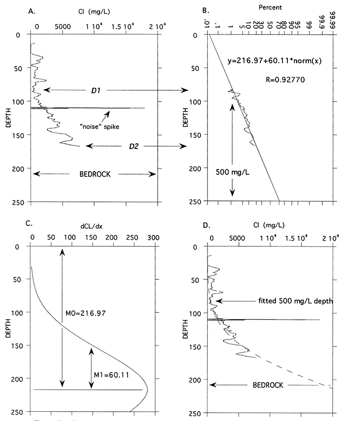
The transition zone region (D1 to D2; Fig. B1A) used for curve fitting was selected by visual inspection of the chloride concentration profile. D1 locates the depth of the deepest portion of the profile consistently below 500 mg/L. D2 is the depth of either the last point on the profile (for incomplete profiles to bedrock) or the depth of the consistently highest concentration on the profile above bedrock. The transition zone region is then plotted on depth-normal probability axes and fitted with a least-squares line (Fig. B1B). The cumulative distribution function is represented by a straight line on the depth-probability axes. The equation for the fitted line, shown on Fig. B1B, contains the mean (M0) as the offset and standard deviation (M1) as the slope that defines the normal distribution of equation 1, is plotted on Fig. B1C, and the cumulative normal distribution shown in Fig. B1D. Because the concentrations are all expressed as a percentage of 42,000 mg/L, the mean (M0) is the depth of the 21,000 mg/L (50%) concentration of the fitted transition zone and the standard deviation (M1) indicates the thickness of the fitted transition zone (M0 + 2M1 = -95% of transition zone area). Because the equation of the curve is fixed, the curve-fitting process can also be adapted to the characterization of the complete transition zone by extension of the fitted line for wells having logs that only partially penetrate the transition zone such as the example from site 11 illustrated in Fig B1.
Figure B1-Example (site 11) of cumulative normal distribution fit to transition zone (TZ). A. DI and D2 indicate range of TZ to be used for fit. TZ is incomplete to bedrock because of well obstruction. B. TZ scaled to percent of 42,000 mg/L and plotted on depth-normal probability axes. Equation of fitted line and correlation coefficient (R) are shown with location of 500 mg/L (1.19%) concentration. C. Normal distribution represented by fitted line in part B: M0 = mean; M1 = standard deviation. D. Cumulative distribution function (dashed line) with chloride concentration profile locates depth of estimated 500 mg/L concentration of TZ and completes TZ profile to bedrock.
The means (M0), standard deviations (M1), and correlation coefficients (R, Fig. B1B) generated by the curve-fitting process represent parameters that characterize the transition zone, along with the actual conductivity values at selected points on the curve. Systematic changes in these parameters represent detectable changes in the freshwater-saltwater transition zone profile. The correlation coefficient (R) indicates the goodness-of-fit of the cumulative distribution function model to the transition zone at each site. The highest values tend to be at sites that generally have large and distinct transitions from fresh to salt water. Weak transition zones are indistinct, noisier, and thus tend to produce lower correlation coefficients. Changes in the correlation coefficient with time may reflect changes in the freshwater-saltwater distribution at a particular site as the transition zone either shifts towards more (increasing R) or less (decreasing R) ideal behavior.
The curve-fitting process allows the elevation of points near the upper and lower extremes of the transition zone to be estimated. For example, the depth of the 500 mg/L level can be estimated from the normal distribution curve fit with the following formula: M0+M1 * NORM(1.19) where M0 and M1 are the mean and standard deviation (Table B1) and NORM(1.19) is the normal distribution function (equation 1) of 500 mg/L expressed as a percentage of 42,000 mg/L (= 1.19%). The values of D1, D2, M0, M1, R, and the depth to the 500 mg/L concentration are tabulated for all sites that have a transition zone in Table B1.
Table B1--Curve-fitting statistics from logs with a transition zone.
| Site | Date | D1 | D2 | M0 (mean) |
M1 (std dev) |
R (corr) |
Depth to 500 mg/L |
Depth change |
|---|---|---|---|---|---|---|---|---|
| 1 | 3/26/93 | 90 | 127.7 | 133.18 | 17.07 | 0.9909 | 94.6 | |
| 1 | 4/15/94 | 90 | 127.7 | 134.54 | 17.894 | 0.9892 | 94.1 | -0.5 |
| 3 | 5/19/93 | 94 | 119 | 197.41 | 43.008 | 0.8229 | 101.15 | |
| 3 | 4/13/94 | 94 | 119 | 192.14 | 39.927 | 0.8102 | 101.85 | 1.7 |
| 4 | 4/22/93 | 80 | 100 | 177.57 | 49.714 | 0.764 | 65.144 | |
| 4 | 4/13/94 | 80 | 100 | 165.23 | 44.262 | 0.8814 | 65.127 | -0.017 |
| 5 | 9/17/93 | 66 | 106 | 98.876 | 12.641 | 0.972 | 68.288 | |
| 5 | 10/16/93 | 66 | 106 | 96.891 | 13.018 | 0.9755 | 67.452 | -0.836 |
| 5 | 4/19/94 | 66 | 106 | 97.269 | 12.539 | 0.9754 | 68.912 | 1.46 |
| 6 | 4/19/93 | bad log data | ||||||
| 6 | 4/13/94 | 78 | 97 | 156.2 | 31.731 | 0.88445 | 84.445 | |
| 8 | 4/21/93 | 500 mg/L set at bedrock depth | 117 | |||||
| 8 | 4/7/94 | 500 mg/L set at bedrock depth | 117 | 0 | ||||
| 9 | 4/25/93 | 40 | 79.5 | 90.065 | 17.336 | 0.5944 | 50.859 | |
| 9 | 4/14/94 | 40 | 79.5 | 88.037 | 16.182 | 0.5655 | 51.442 | 0.583 |
| 10 | 4/18/93 | 111 | 126 | 164.71 | 24.533 | 0.81843 | 109.23 | |
| 10 | 4/7/94 | 111 | 126 | 160.34 | 21.824 | 0.82634 | 110.99 | 1.76 |
| 11 | 3/27/93 | 82 | 167.1 | 216.97 | 60.108 | 0.9277 | 81.038 | |
| 11 | 5/20/93 | 82 | 167.1 | 221.95 | 64.422 | 0.9289 | 76.259 | -4.779 |
| 11 | 7/9/93 | 82 | 167.1 | 220.58 | 63.57 | 0.9286 | 76.819 | 0.56 |
| 11 | 7/30/93 | 82 | 167.1 | 220.22 | 63.285 | 0.9279 | 77.103 | 0.284 |
| 11 | 9/22/93 | 82 | 167.1 | 221.78 | 65.076 | 0.9276 | 74.611 | -2.492 |
| 11 | 10/13/93 | 82 | 167.1 | 221.69 | 65.06 | 0.9291 | 74.56 | -0.051 |
| 11 | 4/8/94 | 82 | 167.1 | 226.16 | 66.184 | 0.912 | 76.429 | 1.869 |
| 16 | 3/25/93 | 122 | 187 | 176.97 | 21.62 | 0.9691 | 128.08 | |
| 16 | 5/19/93 | 122 | 187 | 177.19 | 21.454 | 0.9695 | 128.67 | 0.59 |
| 16 | 7/8/93 | 122 | 187 | 177.19 | 21.757 | 0.9686 | 127.99 | -0.68 |
| 16 | 7/31/93 | 122 | 187 | 176.88 | 22.301 | 0.9734 | 126.44 | -1.55 |
| 16 | 9/8/93 | 122 | 187 | 176.03 | 19.329 | 0.9773 | 132.31 | 5.87 |
| 16 | 10/21/93 | 122 | 187 | 176.88 | 22.319 | 0.9704 | 126.41 | -5.9 |
| 16 | 3/31/94 | 122 | 187 | 176.63 | 21.89 | 0.974 | 127.13 | 0.71999 |
| 17 | 3/25/93 | 61 | 100 | 111.1 | 20.366 | 0.9412 | 65.046 | |
| 17 | 5/19/93 | 61 | 100 | 112.15 | 21.578 | 0.9446 | 63.348 | -1.698 |
| 17 | 7/8/93 | 61 | 100 | 112.49 | 21.759 | 0.9447 | 63.281 | -0.067 |
| 17 | 7/28/93 | 61 | 100 | 112.95 | 22.45 | 0.9455 | 62.178 | -1.103 |
| 17 | 9/8/93 | 61 | 100 | 111.01 | 20.179 | 0.9384 | 65.372 | 3.194 |
| 17 | 10/21/93 | 61 | 100 | 111.08 | 20.447 | 0.9409 | 64.843 | -0.529 |
| 17 | 4/1/94 | 61 | 100 | 111.02 | 20.488 | 0.9395 | 64.681 | -0.162 |
| 18 | 3/25/93 | 107 | 172 | 182.26 | 31.753 | 0.8504 | 110.45 | |
| 18 | 5/21/93 | 107 | 172 | 183.84 | 33.194 | 0.8618 | 108.77 | -1.68 |
| 18 | 7/9/93 | 107 | 172 | 183.09 | 32.716 | 0.85 | 109.1 | 0.33 |
| 18 | 7/29/93 | 107 | 172 | 183 | 32.624 | 0.844 | 109.22 | 0.12 |
| 18 | 10/14/93 | 107 | 172 | 182.55 | 32.282 | 0.8482 | 109.55 | 0.33 |
| 18 | 4/8/94 | 107 | 172 | 181.63 | 31.233 | 0.8407 | 110.99 | 1.44 |
| 19 | 4/19/93 | 142 | 163 | 237.37 | 41.181 | 0.78367 | 144.23 | |
| 19 | 4/7/94 | 142 | 163 | 237.49 | 41.545 | 0.78048 | 143.54 | -0.69 |
| 21 | 5/20/93 | 80 | 136.1 | 161.27 | 34.198 | 0.9653 | 83.934 | |
| 21 | 4/7/94 | 80 | 136.1 | 160.13 | 32.164 | 0.9642 | 87.387 | 3.453 |
| 22 | 3/25/93 | 133 | 204 | 198.15 | 25.648 | 0.9338 | 140.15 | |
| 22 | 5/21/93 | 133 | 204 | 197.44 | 24.721 | 0.944 | 141.53 | 1.38 |
| 22 | 7/9/93 | 133 | 204 | 197.91 | 24.926 | 0.9262 | 141.53 | 0 |
| 22 | 7/30/93 | 133 | 204 | 197.93 | 25.114 | 0.9271 | 141.14 | -0.39 |
| 22 | 10/14/93 | 133 | 204 | 197.08 | 24.427 | 0.938 | 141.84 | 0.7 |
| 22 | 3/31/94 | 133 | 204 | 197.82 | 24.549 | 0.9523 | 142.3 | 0.46001 |
| 23 | 4/20/93 | 52.5 | 82 | 123.87 | 21.585 | 0.5614 | 75.05 | |
| 23 | 4/19/94 | 52.5 | 82 | 158.41 | 40.539 | 0.6778 | 66.732 | -8.318 |
| 24 | 4/20/93 | 88 | 112 | 146.88 | 24.408 | 0.86403 | 91.68 | |
| 24 | 4/19/94 | 88 | 112 | 148.55 | 25.444 | 0.8805 | 91.008 | -0.672 |
| 25 | 3/28/93 | 8 | 38 | 35.675 | 11.43 | 0.9346 | 9.827 | |
| 25 | 7/31/93 | 8 | 38 | 34.896 | 11.427 | 0.901 | 9.053 | -0.774 |
| 25 | 9/14/93 | 8 | 38 | 34.9 | 11.64 | 0.8947 | 8.577 | -0.476 |
| 25 | 10/22/93 | 8 | 38 | 34.91 | 11.568 | 0.8944 | 8.748 | 0.171 |
| 25 | 4/4/94 | 8 | 38 | 35.56 | 11.099 | 0.9477 | 10.46 | 1.712 |
| 26 | 4/20/93 | 64 | 102 | 102.11 | 12.625 | 0.9278 | 73.56 | |
| 26 | 4/15/94 | 64 | 102 | 106.61 | 17.432 | 0.9788 | 67.19 | -6.37 |
| 27 | 4/20/93 | 53 | 66 | 78.229 | 7.5943 | 0.9907 | 61.054 | |
| 27 | 4/15/94 | 53 | 66 | 84.086 | 11.187 | 0.9905 | 58.788 | -2.266 |
| 29 | 4/25/93 | 94 | 150 | 254.31 | 67.954 | 0.634 | 100.64 | |
| 29 | 4/7/94 | 94 | 150 | 248.73 | 64.379 | 0.6457 | 103.13 | 2.49 |
| 30 | 4/25/93 | 85 | 132 | 216.98 | 48.91 | 0.5368 | 106.36 | |
| 30 | 4/14/94 | 85 | 132 | 204.65 | 42.662 | 0.4906 | 108.17 | 1.81 |
| 31 | 4/20/93 | 73 | 90 | 196.27 | 52.737 | 0.8467 | 77.008 | |
| 31 | 4/15/94 | 73 | 90 | 192 | 50.257 | 0.8138 | 78.345 | 1.337 |
| 32 | 4/24/93 | 75 | 135 | 158.26 | 31.292 | 0.6085 | 87.497 | |
| 32 | 4/19/94 | 75 | 135 | 151.87 | 27.745 | 0.551 | 89.126 | 1.629 |
| 33 | 5/20/93 | 120 | 139 | 191.41 | 26.976 | 0.794 | 130.41 | |
| 33 | 4/7/94 | 120 | 139 | 176.71 | 18.718 | 0.8117 | 134.38 | 3.97 |
| 35 | 4/21/93 | 115 | 142 | 186.37 | 27.447 | 0.8686 | 124.3 | |
| 35 | 4/20/94 | 115 | 142 | 188.79 | 28.937 | 0.8685 | 123.34 | -0.96001 |
| 36 | 4/21/93 | 121 | 188 | 202.18 | 31.618 | 0.9544 | 130.67 | |
| 36 | 9/16/93 | 121 | 188 | 199.77 | 28.096 | 0.9635 | 136.23 | 5.56 |
| 36 | 4/14/94 | 121 | 188 | 203.65 | 32.828 | 0.9462 | 129.41 | -6.82 |
| 37 | 4/21/93 | 212 | 233 | 260.55 | 17.497 | 0.902 | 220.98 | |
| 37 | 4/13/94 | 212 | 233 | 259.04 | 16.663 | 0.9271 | 221.36 | 0.38 |
| 38 | 4/21/93 | 150 | 177 | 198.04 | 19.209 | 0.8461 | 154.6 | |
| 38 | 4/14/94 | 150 | 177 | 197.33 | 18.805 | 0.8577 | 154.8 | 0.2 |
| 39 | 10/22/93 | 500 mg/L set at bedrock depth | 55 | |||||
| 39 | 4/20/94 | 500 mg/L set at bedrock depth | 55 | 0 | ||||
| 42 | 4/22/93 | 74 | 149 | 187.52 | 37.412 | 0.93 | 102.91 | |
| 42 | 4/14/94 | 74 | 149 | 188.01 | 37.263 | 0.9392 | 103.74 | 0.82999 |
| 43 | 4/22/93 | 40 | 55 | 61.092 | 7.1996 | 0.9387 | 44.81 | |
| 43 | 4/19/94 | 40 | 55 | 60.55 | 6.8257 | 0.938 | 45.113 | 0.303 |
| 49 | 6/22/94 | 40 | 70 | 87.13 | 17.6 | 0.9264 | 102.7 | |
| SP | 4/17/93 | 123 | 180 | 167.27 | 16.4 | 0.9766 | 130.18 | |
| SP | 5/20/93 | 123 | 180 | 166.63 | 16.224 | 0.9743 | 129.94 | -0.23999 |
| SP | 7/8/93 | 123 | 180 | 166.17 | 15.487 | 0.969 | 131.14 | 1.2 |
| SP | 7/27/93 | 123 | 180 | 166.04 | 14.993 | 0.968 | 132.13 | 0.99001 |
| SP | 7/29/93 | 123 | 180 | 166.09 | 15.343 | 0.9704 | 131.39 | -0.74001 |
| SP | 9/18/93 | 123 | 180 | 166.63 | 17.193 | 0.9702 | 127.75 | -3.64 |
| SP | 10/21/93 | 123 | 180 | 166.46 | 17.707 | 0.9655 | 126.41 | -1.34 |
| SP | 3/24/94 | 123 | 180 | 166.07 | 16.676 | 0.9744 | 128.35 | 1.94 |
| SP | 3/31/94 | 123 | 180 | 166.08 | 16.473 | 0.9753 | 128.82 | 0.47 |
| SP | 4/13/94 | 123 | 180 | 166.01 | 16.166 | 0.97535 | 129.45 | 0.62999 |
| SP | 4/21/94 | 123 | 180 | 166.12 | 16.32 | 0.9752 | 129.21 | -0.23999 |
| SP | 5/19/94 | 123 | 180 | 166.25 | 17.325 | 0.9762 | 127.07 | -2.14 |
| SD | 4/17/93 | 123 | 158.3 | 165.45 | 15.87 | 0.8824 | 129.56 | |
| SD | 5/20/93 | 123 | 158.3 | 164.17 | 15.372 | 0.8888 | 129.41 | -0.14999 |
| SD | 7/8/93 | 123 | 158.3 | 163.97 | 15.389 | 0.8918 | 129.17 | -0.24001 |
| SD | 7/27/93 | 123 | 158.3 | 163.66 | 14.788 | 0.8795 | 130.22 | 1.05 |
| SD | 7/29/93 | 123 | 158.3 | 163.85 | 15.154 | 0.8863 | 129.58 | -0.64 |
| SD | 9/18/93 | 123 | 158.3 | 163.92 | 15.128 | 0.9001 | 129.71 | 0.13 |
| SD | 10/21/93 | 123 | 158.3 | 164.18 | 15.327 | 0.8992 | 129.52 | -0.19 |
| SD | 3/31/94 | 123 | 158.3 | 164.31 | 15.503 | 0.8608 | 129.25 | -0.27 |
| SD | 4/13/94 | 123 | 158.3 | 164.06 | 15.311 | 0.87022 | 129.44 | 0.19 |
| SD | 4/21/94 | 123 | 158.3 | 164.27 | 15.574 | 0.8621 | 129.05 | -0.39 |
| SD | 5/19/94 | 123 | 158.3 | 164.4 | 15.624 | 0.8656 | 129.06 | 0.009995 |
We emphasize that the use of standardized, fitted chloride curves is an empirical approach that supports research purposes and comparisons over time and space. The standardized salinity curves can also be used for salt-budget calculations. However, this approach is not essential to a basic description and understanding of saltwater distribution, and it can not replace interpretation of actual log measurements and chemical analyses in cases of site-specific management and assessment, where the details of the local context will be important.
The basic assumption of the curve fitting process is that the transition zone begins (<500 mg/L) at some point in the aquifer and increases with depth to the bedrock. Therefore, the process can only be successfully applied to logs from sites that have a distinct transition zone (or at least some portion of) that displays this pattern. Sites that are listed as saline transition zone sites in OFR 94-28c that can't be processed by the curve-fitting techniques described above (not included in Table Bl) because they lack data from the necessary transition zone depth range are: 15, 40, and 51.
Deviations from the archetypal transition zone assumption may exist because of incomplete removal of background lithologic contributions to the conductivity signal; "perched" transition zones; or the presence of relatively saltier water in the upper aquifer compared with the lower aquifer possibly from evaporative enrichment, agricultural chemicals, or oil brine contamination. The actual first occurrence of water with a concentration of 500 mg/L may therefore be at a lesser depth than indicated from the curve fitting process because of the ambiguous situations mentioned above. The selection of the depth range to be used for curve fitting (D I to D2) is an attempt to include as much of the profile extending to the bedrock as possible, exclude possible ambiguities, and to maximize (high R value) the fit to a cumulative distribution function. The relative success of the curve fitting process can be assessed by the R value: most sites consistently exceed 0.85; sites where R is less than 0.85 have less distinct and broad (M1 > 40 ft) transition zones that are most subject to distortions due to the presence of ambiguities.
Concentration levels calculated from the fitted profiles, such as the 500 mg/L depth, are intended to represent estimates of idealized, vertically controlled transition zone values as a product of possible hydrodynamic dispersion or diffusion processes starting with an original source brine with a concentration of 42,000 mg/L. The use of 42,000 mg/L chloride as an assumed bedrock limit of the upper end of the transition zone is an estimate based on the limiting concentration. We are aware that in some locations the transition zone extends into the bedrock, and that the actual maximum bedrock concentration may be less than 42,000 mg/L. As part of future work we will explore the effects of this assumption and the utility of alternative approaches. It is presented here as an illustration of the utility of a standardized comparison technique, and an initial estimate of some key parameters. Biases introduced by this assumption should have little effect on the use of the parameters to evaluate changes at a single site. Where the assumption is inaccurate, it will tend to skew the results toward higher salt inventories and sharper transition zones than may actually be the case.
The following sections represent work in progress because the analysis so far has concentrated on sites in the northern Mineral Intrusion study area.
The integrated salt load within the aquifer at each site is determined by calculating the area underneath the chloride concentration profile derived from the corrected conductivity log between the water table (wt) and the bedrock (br). For sites lacking a complete profile to bedrock, the cumulative distribution function fitted to the transition zone (described above) is used to estimate the missing section of the chloride concentration profile. Sites requiring extrapolation of the chloride profile were: 1, 5, 11, and 21. The area (A) was calculated by using the curve integration function in KaleidaGraphtm software running on a Macintosh Quadra. The integrated area (A) under the curve is based on the Riemann sum:
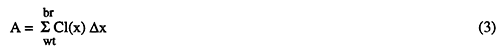
where: Cl(x) is the concentration (mg/L) at depth x, Δx = 0.1 ft, and from the fundamental theorem of calculus:
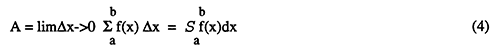
provided that f(x) is continuous and its derivative exists between a and b. The total mass of chloride per unit aquifer surface area is:
Cl(mg/ft2) = 28.32An (5)
where A is the area under the depth profile of chloride concentration (mg-ft/L); 28.32 is a volumetric conversion factor (L/ft3); and n is effective aquifer porosity (unitless; assumed to be 0.16). The total chloride mass is a measure of the salt load for that portion of the aquifer. Table B2 includes the area (A), the chloride mass, and the equivalent saturated thickness at 42,000 mg/L required to equal the mass at sites in the northern part of the study area. Further discussion of these results and their implications will be found in OFR 94-28c and e.
Table B2 part 1--Salt Inventory at some monitoring well sites in the Mineral Intrusion study area (1993).
| Site.well no. | Depth to bedrock |
Depth to water table |
Area under chloride profile |
Chloride mass per unit area |
Equivalent 42k concen. sat. thick |
|---|---|---|---|---|---|
| 1.1 | 146 | 5.3 | 6.43E+05 | 2.91E+06 | 15.308 |
| SP | 186 | 10.8 | 7.96E+05 | 3.60E+06 | 18.94 |
| 3.1 | 130 | 25.73 | 33561 | 1.52E+05 | 0.79907 |
| 4.1 | 129 | 8.7 | 1.91E+05 | 8.66E+05 | 4.5492 |
| 5.1 | 181 | 1.77 | 3.06E+06 | 1.39E+07 | 72.775 |
| 8.1 | 118.3(1) | 8.8 | 68715 | 3.11E+05 | 1.6361 |
| 9.1 | 87 | 9 | 1.96E+05 | 8.89E+05 | 4.6693 |
| 10.1 | 156 | 18.3 | 84985 | 3.85E+05 | 2.0234 |
| 11.1 | 208 | 13.5 | 8.65E+05 | 3.92E+06 | 20.592 |
| 16.1 | 220 | 11.98 | 1.68E+06 | 7.60E+06 | 39.915 |
| 17.1 | 114 | 11.6 | 2.49E+05 | 1.13E+06 | 5.9393 |
| 18.1 | 214 | 19.25 | 8.52E+05 | 3.86E+06 | 20.295 |
| 21.1 | 137 | 21.6 | 2.67E+05 | 1.21E+06 | 6.3524 |
| 22.1 | 215 | 16.1 | 8.07E+05 | 3.66E+06 | 19.208 |
| 23.1 | 94 | 21.42 | 41453 | 1.88E+05 | 0.98698 |
| 24.1 | 123 | 21 | 3.65E+05 | 1.66E+06 | 8.6993 |
| 25.1 | 98 | 6.3 | 1.31E+06 | 5.95E+06 | 31.241 |
| 26.1 | 177 | 6.8 | 9.52E+05 | 4.31E+06 | 22.661 |
| 27.1 | 104 | 10.12 | 82905 | 3.76E+05 | 1.9739 |
| 30.1 | 138 | 14.54 | 56876 | 2.58E+05 | 1.3542 |
| 31.1 | 93 | 13.65 | 37273 | 1.69E+05 | 0.88746 |
| 32.1 | 172 | 2.6 | 2.48E+05 | 1.12E+06 | 5.9067 |
| 36.1 | 195 | 28 | 4.26E+05 | 1.93E+06 | 10.15 |
| 37.1 | 240 | 58.63 | 95705 | 4.34E+05 | 2.2787 |
| 42.1 | 160 | 13.03 | 1.53E+05 | 6.91E+05 | 3.6311 |
| 43.1 | 65 | 4.87 | 71699 | 3.25E+05 | 1.7071 |
| 50.1 | 223 | 26.15 | 13657 | 61885 | 0.32518 |
| 51.1 | 200 | 17.3 | 23314 | 1.06E+05 | 0.5551 |
| 52.1 | 221 | 30.79 | 15816 | 71667 | 0.37658 |
| Notes: (1) Depth to bedrock changed from 117 ft based on inspection of conductivity log. Depths and thicknesses in feet; Area = (mg-ft)/L; Mass (mg/sq. ft). |
|||||
Table B2 part 2--Salt inventory at some monltonnc well sites In the Mineral Intrusion study area (1994).
| Site.well no. | Depth to bedrock |
Depth to water table |
Area under chloride profile |
Chloride mass per unit area |
Equivalent 42k concen. sat. thick |
|---|---|---|---|---|---|
| 1.1 | 146 | 6.35 | 6.10E+05 | 2. 76E+06 | 14.517 |
| SP | 186 | 11.3 | 8.05E+05 | 3.65E+06 | 19.172 |
| 3.1 | 130 | 20.54 | 32818 | 1.49E+05 | 0.78138 |
| 4.1 | 129 | 7.87 | 2.17E+05 | 9.82E+05 | 5.1603 |
| 5.1 | 181 | 2.08 | 3.05E+06 | 1.38E+07 | 72.522 |
| 8.1 | 118.3(1) | 11.1 | 75413 | 3.42E+05 | 1.7955 |
| 9.1 | 87 | 9.36 | 2.07E+05 | 9.39E+05 | 4.9332 |
| 10.1 | 156 | 13.75 | 79998 | 3.62E+05 | 1.9047 |
| 11.1 | 208 | 11.39 | 8.04E+05 | 3.64E+06 | 19.135 |
| 16.1 | 220 | 7.64 | 1.66E+06 | 7.50E+06 | 39.412 |
| 17.1 | 114 | 10.54 | 2.57E+05 | 1.16E+06 | 6.1104 |
| 18.1 | 214 | 11.02 | 8.59E+05 | 3.89E+06 | 20.454 |
| 21.1 | 137 | 23.07 | 2. 16E+05 | 9.80E+05 | 5.1505 |
| 22.1 | 215 | 12.71 | 8.09E+05 | 3.67E+06 | 19.267 |
| 23.1 | 94 | 22.4 | 40763 | 1.85E+05 | 0.97055 |
| 24.1 | 123 | 23.9 | 2.57E+05 | 1.16E+06 | 6.1079 |
| 25.1 | 98 | 6.02 | 1.32E+06 | 6.ooE+06 | 31.535 |
| 26.1 | 177 | 8.76 | 1.03E+06 | 4.66E+06 | 24.47 |
| 27.1 | 104 | 11.22 | 1.09E+05 | 4.92E+05 | 2.5833 |
| 30.1 | 138 | 17.19 | 47496 | 2. 15E+05 | 1.1308 |
| 31.1 | 93 | 15.06 | 35320 | 1.60E+05 | 0.84096 |
| 32.1 | 172 | 9.1 | 2.60E+05 | 1.18E+06 | 6.1963 |
| 36.1 | 195 | 27.84 | 4.30E+05 | 1.95E+06 | 10.249 |
| 37.1 | 240 | 57.1 | 92821 | 4.21E+05 | 2.21 |
| 42.1 | 160 | 13.01 | 1.50E+05 | 6. 79E+05 | 3.5671 |
| 43.1 | 65 | 5.14 | 81034 | 3.67E+05 | 1.9294 |
| 49.1 | 106 | 1 | 196670 | 8.91E+05 | 4.6826 |
| 50.1 | 223 | 22.34 | 14846 | 67271 | 0.35348 |
| 51.1 | 200 | 13.68 | 24149 | 1.09E+05 | 0.57498 |
| 52.1 | 221 | 23.67 | 16859 | 76390 | 0.40139 |
| Notes: (1) Depth to bedrock changed from 117 ft based on inspection of conductivity log. Depths and thicknesses in feet; Area = (mg-ft)/L; mass = (mg/sq. ft). |
|||||
The applications of complete chloride concentration profiles for sites in the Great Bend Prairie aquifer include corrections for density effects on hydraulic head measurements and the determination of total salt mass for a particular site. Density-corrected head measurements will allow the development of an accurate horizontal and vertical component flow field within the aquifer. Together, the flow field and salt inventory will be used to determine the aquifer salt budget for the Mineral Intrusion study area.
Flow-field calculations involving water of high total dissolved solids (TDS) or higher or lower than normal temperatures requires that the effects of density be included in the formulations. For example, a salt water with a TDS of approximately 35,000 mg/L will have a density of 1.025 gm/cm3 as compared to pure water with a density of 0.999973 gm/cm3 at 4 deg C; pure water at 50 deg C has a density of 0.988047 gm/cm3 (Anderson and Woessner, 1992). These seemingly small changes in density can have a significant influence on the flow-field calculations, especially when potentiometric gradients are commensurately small to begin with. However, since the total thickness of the Great Bend Prairie aquifer is relatively small with small changes in temperature, only density variations due to changes in chloride concentration and not temperature need to be considered.
Figure B2 demonstrates the relationship between chloride concentration and density of seawater at 15 deg. C (Williams, 1962), the typical temperature (in situ) of ground water in the Great Bend Prairie aquifer. The linear relationship must be extrapolated to concentrations of 42,000 mg/L (the maximum groundwater concentration) because the relationship was developed for seawater with typical chloride concentrations of less than 25,000 mg/L. Although there are slight differences between the ionic ratios of seawater and of Permian formation brine, they are similar enough to justify the use of this relationship.
Figure B2--Conversion of chloride concentration to density.
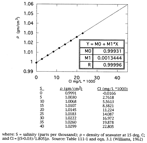
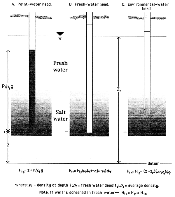
Figure B3 illustrates the concepts of hydraulic heads in variable density situations as described by Lusczynski (1961). The point-water head (Fig. B3A) is the field-measured fluid level, which is assumed to reflect the head of the well filled with water of uniform density equal to that occurring at the depth of the well screen. The fresh-water head (Fig. B3B) is the hypothetical head of the same well filled with uniformly fresh water. The environmental-water head (Fig. B3C) is the hypothetical head of the same well filled with the variable density water reflecting the actual vertical density gradient in the aquifer. The environmental-water correction can also be thought of as the freshwater correction reduced by an amount corresponding to the difference between the salt mass in fresh water and that in the actual (environmental) water in the interval from the top of the zone of saturation to the well screen (Lusczynski, 1961). Because the environmental-water head correction reflects the actual vertical mass distribution in the aquifer and thus an approximation of the density-related, gravity-driven component of flow, this correction is used to calculate vertical gradients within the aquifer.
Figure B3--Heads in ground water of variable density (after Lusczynski, 1961).
For assessing the probable rate of inflow of saltwater from the Permian to the Great Bend Prairie aquifer formations, the critical head gradient is across the bedrock interface. In order to estimate that value on the basis of normalized densities, we use the difference between the calculated freshwater head of the Permian well (Hif, assumed to represent the density-corrected driving force for upward flow) and the environmental head at the bedrock datum (Hin, assumed to represent the density-corrected confining pressure of the overlying water column). These gradients are presented and discussed in reports OFR 94-28d and e.
The environmental head, based on the average density, is calculated quite simply from the integrated chloride profile area A (from eqn. 4 above) by dividing the value of A (mg-ft/L) by the saturated thickness of the aquifer. This provides the average chloride concentration over the depth in question; that value can be transformed into average density using the expression presented in Figure B2.
The results of head corrections for several sites, with measurements from 1993 and 1994, are contained in Table B3 parts 1 and 2. Two examples from Table B3 illustrate the necessity and precision of the head corrections. For site 5, the point-water heads indicate a recharge (downward) potential between the upper (number 3 well) and the lower (number 2 well) aquifer whereas the environmental-water corrected heads indicate a discharge (upward) potential. Because site 5 is located close to the gaining (discharge) Rattlesnake Creek and has an unusually thick and massive salt-water profile (Table B2), a discharge gradient appears to reflect the actual fluid potential within the aquifer. For site 8, the number 2 and 3 wells are both screened in the lower aquifer with approximately 30 ft of depth separation. The point-water heads for these two wells are approximately 0.3 ft different for both 1993 and 1994 measurements whereas the density-corrected heads are brought into coincidence to within 0.06 ft for 1993 and to within 0.01 ft for 1994 -- the much smaller gradients, at site 8, again reflecting congruity of fluid potentials. This high level of precision in matching the corrected heads indicates that very accurate potential flow field calculations, especially critical in the vertical direction within the Mineral Intrusion study area, can be calculated for the Great Bend Prairie aquifer if adequate elevation data are available.
Table B3 part 1--Variable-density head corrections for monitoring well sites in the northern and selected sites in the southern Mineral Intrusion study area 1993).
| Site.well no. | Depth to Bedrock |
Depth to Screen |
Depth to Water Table |
Depth to Water |
Density at Screen (1) |
Average Density (2) |
Point-water Head (3) |
Fresh-water Head |
Environmental- Water Head |
|---|---|---|---|---|---|---|---|---|---|
| 1.1 | 146 | 146 | 5.3 | 6.8 | 1.0171 | 1.0055 | 139.2 | 141.67 | 140.74 |
| 1.2 | 146 | 106 | 5.3 | 5.7 | 1.0036 | 0.99973 | 140.3 | 140.73 | 140.68 |
| 1.3 | 146 | 36 | 5.3 | 5.3 | 0.99936 | 0.9995 | 140.7 | 140.7 | 140.69 |
| SP | 186 | 197 | 10.8 | 20.9 | 1.0352 | 1.0054 | 175.2 | 181.88 | 180.75 |
| 3.1 | 130 | 120 | 25.73 | 28.31 | 1.0135 | 0.99974 | 101.69 | 102.99 | 102.93 |
| 3.2 | 130 | 65 | 25.73 | 25.73 | 0.9994 | 0.99941 | 104.27 | 104.27 | 104.26 |
| 4.1 | 129 | 217 | 8.7 | 5.8 | 1.041 | 1.0015 | 123.2 | 132.01 | 131.51 |
| 4.2 | 129 | 106 | 8.7 | 5.8 | 1.0004 | 1.0013 | 123.2 | 123.31 | 123.08 |
| 4.3 | 129 | 53 | 8.7 | 8.7 | 1.0009 | 1.001 | 120.3 | 120.37 | 120.27 |
| 5.1 | 181 | 193 | 1.77 | 1 | 1.0547 | 1.0222 | 180 | 190.64 | 186.17 |
| 5.2 | 181 | 92 | 1.77 | 3.26 | 1.0282 | 1.0019 | 177.74 | 180.31 | 180.06 |
| 5.3 | 181 | 40 | 1.77 | 1.77 | 0.99936 | 0.99973 | 179.23 | 179.23 | 179.21 |
| 8.1 | 118.3 (4) | 237 | 8.8 | 25.1 | 1.0582 | 1.0002 | 93.2 | 105.69 | 105.48 |
| 8.2 | 118.3 (4) | 116 | 8.8 | 15.8 | 1.0024 | 1.0001 | 102.5 | 102.81 | 102.71 |
| 8.3 | 118.3 (4) | 87 | 8.8 | 15.5 | 1.0001 | 1.0002 | 102.8 | 102.86 | 102.77 |
| 8.4 | 118.3 (4) | 46 | 8.8 | 8.8 | 0.99998 | 0.99955 | 109.5 | 109.52 | 109.51 |
| 9.1 | 87 | 86 | 9 | 9 | 1.0037 | 1.0027 | 78 | 78.34 | 78.018 |
| 9.2 | 87 | 62 | 9 | 8.8 | 1.0012 | 1.0004 | 78.2 | 78.301 | 78.223 |
| 9.3 | 87 | 38 | 9 | 9 | 0.99936 | 0.99955 | 78 | 78.001 | 77.99 |
| 10.1 | 156 | 160 | 18.3 | 22.9 | 1.0016 | 1.0001 | 133.1 | 133.42 | 133.27 |
| 10.2 | 156 | 143 | 18.3 | 22.7 | 1.0013 | 1 | 133.3 | 133.54 | 133.43 |
| 10.3 | 156 | 100 | 18.3 | 20.8 | 1.0004 | 0.99961 | 135.2 | 135.29 | 135.25 |
| 10.4 | 156 | 74 | 18.3 | 18.3 | 0.99961 | 0.99942 | 137.7 | 137.72 | 137.71 |
| 11 .1 | 208 | 237 | 13.5 | 31.89 | 1.0329 | 1.0053 | 176.11 | 183.01 | 181.51 |
| 11.2 | 208 | 61 | 13.5 | 13.5 | 1.0002 | 1.0002 | 194.5 | 194.54 | 194.48 |
| 16.1 | 220 | 243 | 11.98 | 29.2 | 1.0461 | 1.0101 | 190.8 | 200.81 | 198.05 |
| 16.2 | 220 | 198 | 11.98 | 19.25 | 1.0452 | 1.0065 | 200.75 | 208.96 | 207.45 |
| 16.3 | 220 | 80 | 11.98 | 11.98 | 0.99948 | 1.0003 | 208.02 | 208.03 | 207.94 |
| 17.1 | 114 | 129 | 11.6 | 45.7 | 1.0126 | 1.0026 | 68.3 | 69.407 | 68.946 |
| 17.2 | 114 | 102 | 11.6 | 10.8 | 1.0105 | 1.002 | 103.2 | 104.22 | 103.92 |
| 17.3 | 114 | 41 | 11.6 | 11.6 | 0.99936 | 0.99952 | 102.4 | 102.4 | 102.39 |
| 18.1 | 214 | 231 | 19.25 | 34.32 | 1.0157 | 1.0052 | 179.68 | 182.91 | 181.43 |
| 18.2 | 214 | 197 | 19.25 | 32.76 | 1.0189 | 1.004 | 181.24 | 184.46 | 183.44 |
| 18.3 | 214 | 45 | 19.25 | 19.25 | 0.99961 | 0.99961 | 194.75 | 194.76 | 194.74 |
| 21.1 | 137 | 145 | 21.6 | 25.2 | 1.015 | 1.0024 | 111.8 | 113.69 | 113.17 |
| 21.2 | 137 | 113 | 21.6 | 22.9 | 1.0047 | 1.0007 | 114.1 | 114.59 | 114.4 |
| 21.3 | 137 | 43 | 21.6 | 21.6 | 1.0003 | 1.0013 | 115.4 | 115.42 | 115.29 |
| 22.1 | 215 | 231 | 16.1 | 29.3 | 1.043 | 1.0048 | 185.7 | 194.52 | 193.17 |
| 22.2 | 215 | 206 | 16.1 | 24.7 | 1.0313 | 1.0036 | 190.3 | 196.1 | 195.15 |
| 22.3 | 215 | 35 | 16.1 | 16.1 | 0.99936 | 0.99936 | 198.9 | 198.9 | 198.9 |
| 23.1 | 94 | 122 | 21.42 | 24.22 | 1.008 | 1.0001 | 69.78 | 70.632 | 70.522 |
| 23.2 | 94 | 79 | 21.42 | 22.99 | 0.99995 | 1 | 71.01 | 71.046 | 70.977 |
| 23.3 | 94 | 44 | 21.42 | 21.42 | 0.99936 | 1.0008 | 72.58 | 72.581 | 72.484 |
| 24.1 | 123 | 131 | 21 | 23.8 | 1.0018 | 1.0041 | 99.2 | 99.462 | 98.73 |
| 24.2 | 123 | 86 | 21 | 21.2 | 0.99997 | 1.0056 | 101.8 | 101.84 | 101.17 |
| 25.1 | 98 | 120 | 6.3 | 11.4 | 1.0227 | 1.0185 | 86.6 | 89.142 | 86.711 |
| 25.2 | 98 | 95 | 6.3 | 12 | 1.0343 | 1.0181 | 86 | 88.906 | 87.001 |
| 25.3 | 98 | 44 | 6.3 | 6.3 | 1.0266 | 1.0123 | 91.7 | 92.73 | 92.076 |
| 26.1 | 177 | 190 | 6.8 | 16.2 | 1.0174 | 1.0068 | 160.8 | 163.95 | 162.47 |
| 26.2 | 177 | 118 | 6.8 | 11 .1 | 1.0154 | 1.0038 | 165.9 | 167.62 | 167.06 |
| 26.3 | 177 | 60 | 6.8 | 6.8 | 0.99961 | 0.99963 | 170.2 | 170.22 | 170.19 |
| 27.1 | 104 | 115 | 10.12 | 10.75 | 1.0018 | 1.0005 | 93.25 | 93.508 | 93.36 |
| 27.2 | 104 | 60 | 10.12 | 10.1 | 1.0005 | 1.0001 | 93.9 | 93.959 | 93.904 |
| 27.3 | 104 | 30 | 10.12 | 10.12 | 0.99994 | 1.0008 | 93.88 | 93.893 | 93.833 |
| 30.1 | 138 | 155 | 14.54 | 17.3 | 1.0026 | 0.99993 | 120.7 | 121.15 | 121.04 |
| 30.2 | 138 | 123 | 14.54 | 14.57 | 1.0003 | 0.99986 | 123.43 | 123.54 | 123.46 |
| 30.3 | 138 | 60 | 14.54 | 14.54 | 0.99936 | 0.99993 | 123.46 | 123.46 | 123.42 |
| 31.1 | 93 | 108 | 13.65 | 13.43 | 1.0017 | 0.99994 | 79.57 | 79.795 | 79.718 |
| 31.2 | 93 | 85 | 13.65 | 13.78 | 1.0004 | 0.9999 | 79.22 | 79.298 | 79.239 |
| 31.3 | 93 | 55 | 13.65 | 13.65 | 1.0002 | 0.99941 | 79.35 | 79.387 | 79.38 |
| 32.1 | 172 | 189 | 2.6 | 45.83 | 1.0018 | 1.0013 | 126.17 | 126.53 | 126.15 |
| 32.2 | 172 | 161 | 2.6 | 45.88 | 1.0022 | 1.0012 | 126.12 | 126.45 | 126.14 |
| 32.3 | 172 | 113 | 2.6 | 1.48 | 1.0025 | 1.0004 | 170.52 | 170.88 | 170.75 |
| 32.4 | 172 | 78 | 2.6 | 2.6 | 1.0002 | 0.99968 | 169.4 | 169.47 | 169.44 |
| 36.1 | 195 | 210 | 28 | 29.9 | 1.0286 | 1.0027 | 165.1 | 170.38 | 169.56 |
| 36.2 | 195 | 191 | 28 | 27.8 | 1.022 | 1.0023 | 167.2 | 170.91 | 170.25 |
| 36.3 | 195 | 146 | 28 | 26 | 1.0026 | 1 | 169 | 169.4 | 169.27 |
| 36.4 | 195 | 85 | 28 | 28 | 1.0004 | 0.99969 | 167 | 167.06 | 167.02 |
| 37.1 | 240 | 255 | 58.63 | 60.84 | 1.0024 | 1 | 179.16 | 179.76 | 179.54 |
| 37.2 | 240 | 235 | 58.63 | 1.0023 | 0.99996 | ||||
| 37.3 | 240 | 151 | 58.63 | 59.06 | 0.99947 | 0.99972 | 180.94 | 180.95 | 180.87 |
| 37.4 | 240 | 82 | 58.63 | 58.63 | 0.99951 | 0.99983 | 181.37 | 181.37 | 181.3 |
| 42.1 | 160 | 178 | 13.03 | 21.28 | 1.0059 | 1.0007 | 138.72 | 139.75 | 139.49 |
| 42.2 | 160 | 157 | 13.03 | 20.36 | 1.0042 | 1.0006 | 139.64 | 140.31 | 140.09 |
| 42.3 | 160 | 103 | 13.03 | 13.03 | 1.0007 | 0.99948 | 146.97 | 147.1 | 147.08 |
| 43.1 | 65 | 88 | 4.87 | 5.4 | 1.0023 | 1.0009 | 59.6 | 59.844 | 59.695 |
| 43.2 | 65 | 40 | 4.87 | 4.87 | 0.9996 | 0.99946 | 60.13 | 60.14 | 60.133 |
| 50.1 | 223 | 190 | 26.15 | 25.94 | 0.99952 | 0.9994 | 197.06 | 197.09 | 197.07 |
| 50.2 | 223 | 120 | 26.15 | 26.09 | 0.99936 | 0.99943 | 196.91 | 196.91 | 196.9 |
| 50.3 | 223 | 45 | 26.15 | 26.15 | 0.99936 | 0.99956 | 196.85 | 196.85 | 196.83 |
| 51.1 | 200 | 170 | 17.3 | 17.83 | 1.0011 | 0.99948 | 182.17 | 182.45 | 182.41 |
| 51.2 | 200 | 95 | 17.3 | 17.3 | 0.99941 | 0.99954 | 182.7 | 182.71 | 182.68 |
| 52.1 | 221 | 195 | 30.79 | 30.4 | 0.99952 | 0.99942 | 190.6 | 190.63 | 190.61 |
| 52.2 | 221 | 97 | 30.79 | 30.79 | 0.99954 | 0.99943 | 190.21 | 190.23 | 190.21 |
| Notes: (1) Median density across screened interval from processed loa profiles except for wells screened in bedrock (Depth to Screen > Depth to Bedrock) where density is calculated from chloride concentration reported by Whittemore (1993). (2) Average density calculated between water table and smaller of screen and bedrock depths. (3) Bedrock depth used for datum at each site. (4) Depth to bedrock changed from 117 ft based on inspection of conductivity log. |
|||||||||
Table 83 part 2--Variable-density head corrections for monitoring well sites in the northern and selected sites in the southern Mineral Intrusion study area (1994).
| Site.well no. | Depth to Bedrock |
Depth to Screen |
Depth to Water Table |
Depth to Water |
Density at Screen (1) |
Average Density (2) |
Point-water Head (3) |
Fresh-water Head |
Environmental- Water Head |
|---|---|---|---|---|---|---|---|---|---|
| 1.1 | 146 | 146 | 6.35 | 6 | 1.0171 | 1.0052 | 140 | 142.49 | 141.59 |
| 1.2 | 146 | 106 | 6.35 | 6.51 | 1.0036 | 0.99973 | 139.49 | 139.92 | 139.87 |
| 1.3 | 146 | 36 | 6.35 | 6.35 | 0.99936 | 0.99945 | 139.65 | 139.65 | 139.65 |
| SP | 186 | 197 | 11.3 | 18.4 | 1.0352 | 1.0055 | 174.7 | 181.36 | 180.22 |
| 3.1 | 130 | 120 | 20.54 | 23.31 | 1.0117 | 0.99971 | 106.69 | 107.89 | 107.83 |
| 3.2 | 130 | 65 | 20.54 | 20.54 | 0.99939 | 0.99941 | 109.46 | 109.46 | 109.46 |
| 4.1 | 129 | 217 | 7.87 | 5.54 | 1.041 | 1.0017 | 123.46 | 132.28 | 131.74 |
| 4.2 | 129 | 106 | 7.87 | 3.16 | 1.0012 | 1.0015 | 125.84 | 126.03 | 125.78 |
| 4.3 | 129 | 53 | 7.87 | 7.87 | 1.001 | 1.0011 | 121.13 | 121.21 | 121.1 |
| 5.1 | 181 | 193 | 2.08 | 1.53 | 1.0547 | 1.0222 | 179.47 | 190.08 | 185.62 |
| 5.2 | 181 | 92 | 2.08 | 3.6 | 1.028 | 1.0017 | 177.4 | 179.94 | 179.71 |
| 5.3 | 181 | 40 | 2.08 | 2.08 | 0.99936 | 0.99955 | 178.92 | 178.92 | 178.91 |
| 8.1 | 118.3 (4) | 237 | 11 .1 | 23.52 | 1.0582 | 1.0003 | 94.78 | 107.36 | 107.12 |
| 8.2 | 118.3 (4) | 116 | 11 .1 | 17.19 | 1.0032 | 1.0002 | 101.11 | 101.49 | 101.38 |
| 8.3 | 118.3 (4) | 87 | 11.1 | 16.86 | 0.99999 | 1.0003 | 101.44 | 101.49 | 101.39 |
| 8.4 | 118.3 (4) | 46 | 11.1 | 11 .1 | 0.99998 | 0.99955 | 107.2 | 107.22 | 107.21 |
| 9.1 | 87 | 86 | 9.36 | 9.34 | 1.0037 | 1.0029 | 77.66 | 77.998 | 77.656 |
| 9.2 | 87 | 62 | 9.36 | 9.2 | 1.0013 | 1.0003 | 77.8 | 77.905 | 77.834 |
| 9.3 | 87 | 38 | 9.36 | 9.36 | 0.99936 | 0.99944 | 77.64 | 77.641 | 77.635 |
| 10.1 | 156 | 160 | 13.75 | 20.4 | 1.0016 | 1.0001 | 135.6 | 135.92 | 135.79 |
| 10.2 | 156 | 143 | 13.75 | 20.16 | 1.0012 | 0.99995 | 135.84 | 136.07 | 135.97 |
| 10.3 | 156 | 100 | 13.75 | 18.12 | 1.0003 | 0.99959 | 137.88 | 137.96 | 137.93 |
| 10.4 | 156 | 74 | 13.75 | 13.75 | 0.99956 | 0.99942 | 142.25 | 142.27 | 142.26 |
| 11.1 | 208 | 237 | 11.39 | 29.37 | 1.0329 | 1.0048 | 178.63 | 185.61 | 184.25 |
| 11.2 | 208 | 61 | 11.39 | 11.39 | 1.0003 | 1.0003 | 196.61 | 196.66 | 196.59 |
| 16.1 | 220 | 243 | 7.64 | 20.85 | 1.0461 | 1.0098 | 199.15 | 209.55 | 206.92 |
| 16.2 | 220 | 198 | 7.64 | 14.93 | 1.0445 | 1.0063 | 205.07 | 213.35 | 211.91 |
| 16.3 | 220 | 80 | 7.64 | 7.64 | 0.99936 | 0.99982 | 212.36 | 212.36 | 212.32 |
| 17.1 | 114 | 129 | 10.54 | 44.06 | 1.0126 | 1.0026 | 69.94 | 71.069 | 70.603 |
| 17.2 | 114 | 102 | 10.54 | 9.91 | 1.0106 | 1.002 | 104.09 | 105.13 | 104.83 |
| 17.3 | 114 | 41 | 10.54 | 10.54 | 0.99936 | 0.99954 | 103.46 | 103.46 | 103.45 |
| 18.1 | 214 | 231 | 11.02 | 26.44 | 1.0157 | 1.005 | 187.56 | 190.92 | 189.54 |
| 18.2 | 214 | 197 | 11.02 | 26.97 | 1.0192 | 1.0038 | 187.03 | 190.41 | 189.48 |
| 18.3 | 214 | 45 | 11.02 | 11.02 | 0.99957 | 0.99954 | 202.98 | 202.99 | 202.98 |
| 21.1 | 137 | 145 | 23.07 | 26.04 | 1.015 | 1.0019 | 110.96 | 112.83 | 112.4 |
| 21.2 | 137 | 113 | 23.07 | 23.93 | 1.0042 | 1.0004 | 113.07 | 113.51 | 113.36 |
| 21.3 | 137 | 43 | 23.07 | 23.07 | 0.99999 | 1.0008 | 113.93 | 113.94 | 113.85 |
| 22.1 | 215 | 231 | 12.71 | 24.57 | 1.043 | 1.0047 | 190.43 | 199.46 | 198.14 |
| 22.2 | 215 | 206 | 12.71 | 20.11 | 1.0305 | 1.0035 | 194.89 | 200.69 | 199.77 |
| 22.3 | 215 | 35 | 12.71 | 12.71 | 0.99936 | 0.99936 | 202.29 | 202.29 | 202.29 |
| 23.1 | 94 | 122 | 22.4 | 23.93 | 1.008 | 1.0001 | 70.07 | 70.925 | 70.814 |
| 23.2 | 94 | 79 | 22.4 | 21.95 | 1.0006 | 0.99969 | 72.05 | 72.124 | 72.085 |
| 23.3 | 94 | 44 | 22.4 | 22.4 | 0.99939 | 0.99942 | 71.6 | 71.602 | 71.594 |
| 24.1 | 123 | 131 | 23.9 | 25.94 | 1.0018 | 1.0028 | 97.06 | 97.317 | 96.778 |
| 24.2 | 123 | 86 | 23.9 | 24.15 | 0.99991 | 1.0036 | 98.85 | 98.887 | 98.415 |
| 25.1 | 98 | 120 | 6.02 | 11.8 | 1.0227 | 1.0187 | 86.2 | 88.733 | 86.292 |
| 25.2 | 98 | 95 | 6.02 | 12.64 | 1.0318 | 1.0182 | 85.36 | 88.038 | 86.128 |
| 25.3 | 98 | 44 | 6.02 | 6.02 | 1.0267 | 1.0121 | 91.98 | 93.021 | 92.381 |
| 26.1 | 177 | 190 | 8.76 | 16.72 | 1.0174 | 1.0075 | 160.28 | 163.42 | 161.79 |
| 26.2 | 177 | 118 | 8.76 | 12.61 | 1.0166 | 1.0042 | 164.39 | 166.21 | 165.59 |
| 26.3 | 177 | 60 | 8.76 | 8.76 | 0.99994 | 0.99983 | 168.24 | 168.27 | 168.24 |
| 27.1 | 104 | 115 | 11.22 | 11.52 | 1.0018 | 1.0009 | 92.48 | 92.736 | 92.538 |
| 27.2 | 104 | 60 | 11.22 | 11.05 | 1.0008 | 1.0004 | 92.95 | 93.023 | 92.945 |
| 27.3 | 104 | 30 | 11.22 | 11.22 | 1.0002 | 1.0013 | 92.78 | 92.797 | 92.715 |
| 30.1 | 138 | 155 | 17.19 | 18.59 | 1.0026 | 0.99984 | 119.41 | 119.85 | 119.76 |
| 30.2 | 138 | 123 | 17.19 | 17.15 | 1.0002 | 0.99976 | 120.85 | 120.94 | 120.88 |
| 30.3 | 138 | 60 | 17.19 | 17.19 | 0.99937 | 0.99974 | 120.81 | 120.81 | 120.78 |
| 31.1 | 93 | 108 | 15.06 | 14.3 | 1.0017 | 0.99992 | 78.7 | 78.923 | 78.848 |
| 31.2 | 93 | 85 | 15.06 | 14.6 | 1.0004 | 0.99988 | 78.4 | 78.477 | 78.42 |
| 31.3 | 93 | 55 | 15.06 | 15.06 | 0.99998 | 0.9994 | 77.94 | 77.967 | 77.96 |
| 32.1 | 172 | 189 | 9.1 | 48.64 | 1.0018 | 1.0015 | 123.36 | 123.71 | 123.29 |
| 32.2 | 172 | 161 | 9.1 | 47.87 | 1.0023 | 1.0014 | 124.13 | 124.47 | 124.11 |
| 32.3 | 172 | 113 | 9.1 | 4.95 | 1.0026 | 1.0006 | 167.05 | 167.41 | 167.25 |
| 32.4 | 172 | 78 | 9.1 | 9.1 | 1.0003 | 0.99981 | 162.9 | 162.97 | 162.92 |
| 36.1 | 195 | 210 | 27.84 | 28.43 | 1.0286 | 1.0028 | 166.57 | 171.9 | 171.07 |
| 36.2 | 195 | 191 | 27.84 | 27.65 | 1.0193 | 1.0024 | 167.35 | 170.62 | 169.94 |
| 36.3 | 195 | 146 | 27.84 | 24.83 | 1.0026 | 1.0001 | 170.17 | 170.57 | 170.43 |
| 36.4 | 195 | 85 | 27.84 | 27.84 | 1.0001 | 0.99971 | 167.16 | 167.21 | 167.16 |
| 37.1 | 240 | 255 | 57.1 | 59.09 | 1.0024 | 0.99999 | 180.91 | 181.52 | 181.31 |
| 37.2 | 240 | 235 | 57.1 | 1.0022 | 0.99993 | ||||
| 37.3 | 240 | 151 | 57.1 | 57.53 | 0.99944 | 0.99971 | 182.47 | 182.48 | 182.4 |
| 37.4 | 240 | 82 | 57.1 | 57.1 | 0.99944 | 0.99984 | 182.9 | 182.9 | 182.83 |
| 42.1 | 160 | 178 | 13.01 | 18.48 | 1.0059 | 1.0007 | 141.52 | 142.57 | 142.31 |
| 42.2 | 160 | 157 | 13.01 | 17.61 | 1.0039 | 1.0006 | 142.39 | 143.03 | 142.81 |
| 42.3 | 160 | 103 | 13.01 | 13.01 | 1.0006 | 0.99947 | 146.99 | 147.11 | 147.09 |
| 43.1 | 65 | 88 | 5.14 | 5.19 | 1.0023 | 1.0011 | 59.81 | 60.055 | 59.885 |
| 43.2 | 65 | 40 | 5.14 | 5.14 | 0.99955 | 0.99979 | 59.86 | 59.868 | 59.847 |
| 50.1 | 223 | 190 | 22.34 | 22.2 | 0.99952 | 0.99943 | 200.8 | 200.84 | |
| 50.2 | 223 | 120 | 22.34 | 22.29 | 0.99936 | 0.99946 | 200.71 | 200.71 | 200.69 |
| 50.3 | 223 | 45 | 22.34 | 22.34 | 0.99936 | 0.99956 | 200.66 | 200.66 | 200.64 |
| 51.1 | 200 | 170 | 13.68 | 14.17 | 1.0011 | 0.99948 | 185.83 | 186.11 | 186.08 |
| 51.2 | 200 | 95 | 13.68 | 13.68 | 0.99941 | 0.99954 | 186.32 | 186.33 | 186.3 |
| 52.1 | 221 | 195 | 23.67 | 28.83 | 0.99952 | 0.99942 | 192.17 | 192.2 | 192.18 |
| 52.2 | 221 | 97 | 23.67 | 23.67 | 0.9995 | 0.99945 | 197.33 | 197.34 | 197.33 |
| Notes: (1) Median density across screened interval from processed loa profiles except for wells screened in bedrock (Depth to Screen > Depth to Bedrock) where density is calculated from chloride concentration reported by Whittemore (1993). (2) Average density calculated between water table and smaller of screen and bedrock depths. (3) Bedrock depth used for datum at each site. (4) Depth to bedrock changed from 117 ft based on inspection of conductivity log. |
|||||||||
Anderson, M.P., and W. W. Woessner. 1992. Applied Groundwater Modeling--Simulation of Flow and Advective Transport: Academic Press, Inc., New York. 381 p.
Buddemeier, R. W., M. A. Sophocleous and D. O. Whittemore. 1992. Mineral Intrusion--Investigation of Salt Contamination of Groundwater in the Eastern Great Bend Prairie Aquifer: Kansas Geological Survey, Open-File Report 92-25, 45 pp. [available online]
Domenico, P. A., and F. W. Schwartz. 1990. Physical and Chemical Hydrogeology: John Wiley and Sons, New York. 824 p.
Lusczynski, N. J. 1961. Head and flow of ground water of variable density: Jour. Geophys. Res., v. 66, n. 12, pp. 4247-4256.
Schmorak, S., and A. Mercado. 1969. Upconing of freshwater-seawater interface below pumping wells.: Water Resources Res., v. 5, p. 1290-1311.
Whittemore, D.O. 1993. Ground-water geochemistry in the mineral intrusion area of Groundwater Management District No. 5, south-central Kansas: Kansas Geological Survey, Open-File Report 93-2. [available online]
Williams, J. 1962. Oceanography: Little, Brown and Co., Boston.
Young, D. P., G. W. Garneau, R. W. Buddemeier, D. Zehr, and J. Lanterman. 1993. Elevation and variability of the freshwater-saltwater interface in the Great Bend Prairie aquifer, south-central Kansas: Kansas Geological Survey, Open-File Report 93-55.
Kansas Geological Survey, Geohydrology
Placed online Feb. 18, 2016; originally released Dec., 1994
Comments to webadmin@kgs.ku.edu
The URL for this page is http://www.kgs.ku.edu/Hydro/Publications/1994/OFR94_28b/index.html