|
|
|
|
Progress Report on Preliminary Interpretation and the Third Monitoring 3-D Seismic Survey |
|
|
|||
To date the seismic data from the baseline survey (November 2003) and first two monitoring surveys (January and March 2004) have undergone preliminary processing and very rudimentary interpretations (Sec. I). Over the period June 23-July 1 the third monitoring 3-D seismic survey was conducted to obtain a snapshot before the flood begins a WAG (water-alternating-gas) program (Sec. II).
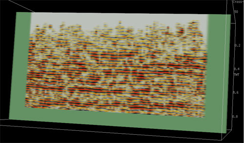
Even at this early stage in the project, post-stack processing of the seismic volumes is providing results that are both encouraging and somewhat unexpected. Significant early pre-stack processing problems related to long-offset NMO stretch, multiples, statics, and reduced resolution for far offsets have been, for the most part, overcome. CMP stacked volumes now possess excellent coherency, with a well defined and detailed velocity function, and near-surface static problems have been all but eliminated (Figure 1). Improvements in the processing flow and parameters are still being made, but the data are ready for preliminary interpretations, including some first-order attribute analysis.
Figure 1--2-D CMP stacked section extracted from 3-D volume of the second monitor survey. Reflection coherency is very good. Improvement in bandwidth and coherency of shallower reflections will be the primary focus of the next round of processing enhancements. A larger version of this figure is available.
Synthetic seismic data derived from sonic logs taken in wells CO2I#1 and #16 will provide essential ties between time on seismic sections and depth on borehole logs. Preliminary correlations between synthetics and real data have been excellent, with convincing matches between the real and synthetic seismic data in proximity to CO2I#1 (Figure 2). Once the higher frequency reflections are enhanced and the dominant frequency moves over 100 Hz at the target depth, final synthetics will be produced allowing identification of the L-KC "C" to an accuracy of around one sample or 10 ft.
Figure 2--Synthetic seismogram generated from a sonic log from CO2I#1 convolved with a Klauder wavelet. The tie between the synthetic and real are outstanding at these lower frequencies. As spectral enhancements are complete the dominant frequency and resolution will increase significantly. A larger version of this figure is available.
Key to many seismic analysis techniques and essential for attribute analysis is the preservation of amplitude, frequency, and phase of the reflected signature. All contributions from the seismic source and noise sources must be reduced as much as possible and ideally eliminated. The reflection signature left on CMP stacked sections must have characteristics that are as closely related to the reflected interface alone as possible without contributions from source, near surface, or background noise (both random and periodic). Considering the comparatively close offset range of interest for these relatively shallow reflections (by industry standards), a significant amount of ground roll and air-coupled wave was removed during processing, leaving some CMP bins with very low fold for some near offset ranges. Removal of multiples is also an important step for optimizing the analysis of these data, because changes in reflection characteristics related to the presence of CO2 in comparison to reservoir fluids are small (approximately 2-20% percent). These data have undergone an extensive series of noise reduction steps to maximize the signal-to-noise ratio and statics/velocity corrections to improve coherency (Figure 3). More work needs to be done to verify that key attributes (phase, frequency, and amplitude) have been preserved up to this point in the processing flow.
Figure 3--2-D slice of 3-D volume with wiggle trace amplitudes represented in color. Coherency is quite good, but work is still underway to insure true amplitudes have been preserved through all processing steps. A few amplitude anomalies resulting from previous work eliminating noise can still be observed on this section. A larger version of this figure is available.
Instantaneous attributes are measurements of specific seismic properties at an instant in time. Measurements of this type are only reliable and useful in extracting meaningful geologic characteristics if all phase and amplitude information is preserved during processing. Multiples and random noise limit the accuracy of interpretations derived from instantaneous attributes.
Given the areal size of the site, it is important to consider the horizontal resolution of the data in interpretations of map view representations of instantaneous attributes. Using the Fresnel zone as the basis for establishing horizontal sampling size on a layer, at 2,900 ft below ground surface for the observed frequencies the radius of the Fresnel zone (generally assumed to be the wavelet sampling size) is approximately 350 ft. Bin (cell) dimensions for these attribute data are approximately 30 ft x 30 ft with a unique value for each cell that includes variable contribution from the surrounding 50 or so cells or ~5 cells away in any direction. Therefore, even though the greatest contributions to each cell's value are from rocks within that cell area, nearby rocks outside the bin are influencing this value to some degree. Interpretations of patterns or textures must consider the overall sampling size of the wavelet and how far from the cell changes in rock property are contributing to the overall signature.
In this document well locations are based on conversions from legal descriptions assigned during the permitting process when the wells were initially drilled. Therefore exact plotted locations relative to this DGPS (less than 0.25 m) seismic grid could be in error by 50 ft or more (up to several cells). DGPS locations of the wells were obtained following the third survey and will be utilized in future analysis but are not shown in the figures here.
Interpretation of the seismic response, particularly for reservoir properties and fluid property changes, involves analysis of numerous attributes of the seismic waveforms returning from the subsurface and specifically from the single wavelet (peak and trough) that sampled the LKC "C" zone. With only the uphole data from #16 available (synthetics [Figure 2] and VSP are not fully developed yet) for time-to-depth correlation of reflections with reflectors, it is not yet possible to confidently identify the exact wavelet returning from the L-KC "C". When the synthetics are fully developed and confidently matched with the real data the exact reflection horizon corresponding to the "C" zone will be mapped and attribute analysis will be performed specifically on the "C" zone reflection. Analysis to date has identified a zone or layer 24 msec (100 ft) thick, which includes the horizon of interest. Preliminary post-stack analysis of the seismic time-slice calculated to contain the "C" zone has been performed to investigate and uniquely identify any changes in response within this volume between the baseline and the subsequent two monitor surveys.
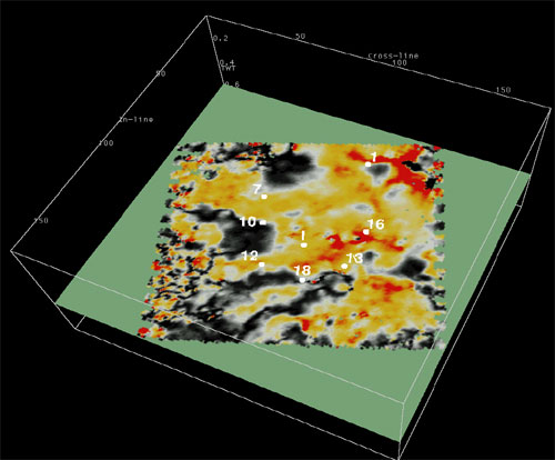
Instantaneous amplitude (amplitude constant-time slice) is the most intuitive of the instantaneous attributes; it provides a measure of reflectivity that represents a map view of seismic amplitude changes. In the case of these 3-D seismic volumes, an instantaneous amplitude time slice provides a general measure of layer structural/depositional topography more than reflectivity, assuming the velocity along the time slice does not vary significantly. From well data within the 4-D seismic area, the L-KC "C" zone exhibits approximately 35 ft of relief between a low near Colliver #6 and high near Colliver # 8. Structurally, Colliver #5 and #6 (west end of survey area) are drilled into lows and Colliver #16, #13, and #8 (eastern end of survey area) are all in a relatively high area. In general, these changes in elevation measured in the well bores are consistent with the amplitude trends on the 560 msec amplitude time slice (Figure 4). Considering this is a time slice and not a horizon map, variations in color are most sensitive to movement of the wavelet up and down in response to changes in reflector depth with only minor contributions from changes in layer reflectivity. Correlation between L-KC "C" elevation and amplitude values is excellent. Work continues trying to map geological/rock-property discontinuities using seismic continuity/similarity volume attributes, which highlight geological discontinuities potentially affecting CO2 movement through the reservoir.
Figure 4A--Color representation of amplitude values along the 560 msec time slice. Dark areas are relative lows and reds are structural highs trending into yellows representative of intermediate depths. A larger version of this figure is available.
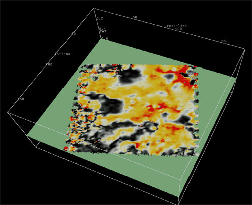
Figure 4B--Same plot with wells located. A larger version of this figure is available.
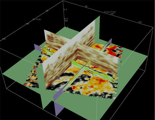
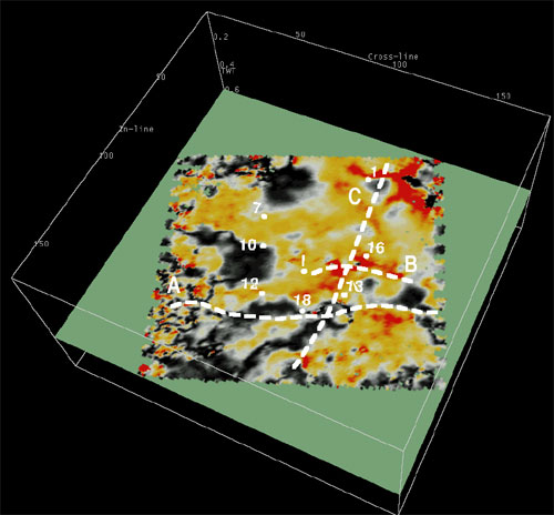
During final data analysis many different visualizations will be necessary to interpret the subtle changes expected from replacement of reservoir fluids (oil and water) with CO2. In-line and cross-line seismic sections are used to calculate various seismic attribute volumes and provide the anchor for studying changes in key time slices and horizons throughout the volume. This analysis approach provides the 3-D visualization utilized to track CO2 movement and geological spatial extent of structural, stratigraphic, and lithologic seismic signatures (Figure 5). Data coherency and uniformity in amplitude characteristics are excellent throughout the interval of interest. Processing to date has focused on the 400-to-700 msec time/depth window. As is evident on shot gathers, many reflections were recorded both shallower and deeper than this interval, and these extraneous reflections will be the target of enhancement processing once the preliminary analysis is complete on the principle zone of interest.
Figure 5--Vertical cross-line and in-line color wiggle trace displays intersected by the 2-D time slice from near the L-KC "C" interval. Correlating the time slice with reservoir tops as defined by well logs results in an excellent match between structure and amplitude. Reds are structurally higher than yellows, which are then higher than the blacks. Average instantaneous frequency in-line and cross-line sections (low is green and high is red) for a sub-volume around the target zone is shown. A larger version of this figure is available.
Preliminary processing of the first three surveys (baseline and two monitor) has provided crude time lapse analysis and shows changes between the baseline survey and the two surveys obtained after CO2 injection began in December 2003. Some of these changes in seismic response can be interpreted to relate to changes in reservoir properties. As noted, with only the uphole data from #16 currently available for time-to-depth correlation of reflections with reflectors, it is not yet possible to confidently identify the exact reflection wavelet that has returned from the L-KC "C". However, a zone or layer 24 msec (100 ft) thick has been selected which includes the horizon of interest. Since the zone of interest (L-KC "C") is only 15% of the total thickness (15 ft of the 100 ft thick time slice) being analyzed, and the change in reflectivity associated with the fluid change from water/oil to CO2 is expected to be less than 20%, changes in seismic properties resulting from the presence of CO2 should be less than 4%. A change in the seismic response this small is at the detection limits of this thick slice analysis technique. It is therefore imperative for accurate interpretation that the exact horizon of interest be identified and analysis be focused on that interval.
A critical processing step that has yet to be performed on these seismic data is equalization. Ground conditions, and therefore coupling and velocity, change over time, resulting in data differences related to what is happening on the ground rather than in the ground. Even with the extreme care taken during acquisition to insure all equipment, parameters, and station locations were identical between surveys, minor changes in surface conditions between the different data acquisition campaigns affect each data set differently. Therefore, corrections unique to each survey data set must be made to reduce and hopefully eliminate surface effects that vary with climate from subsurface effects. After equalization, characteristics of resulting data sets can be directly compared and differenced data sets can be used to highlight CO2 movement. It is important to note that since the data equalization processing has not been completed some of the differences observed between surveys are likely from changes in surface conditions and not changes that occurred in the subsurface.
Instantaneous frequency (IF) analysis was performed on the 24 msec-thick seismic volume. IF is an attribute sensitive to the temporal change in the continuity of seismic events, specifically; it is sensitive to waveform characteristic changes resulting from velocity and/or thickness variations in a thin layer. In general terms it can be considered a measure of seismic spectral attenuation within a rock layer. IF plots by nature tend to have a high degree of variability. Although lateral changes in rock lithology are detectable using IF analysis, numerous different kinds of lithologic changes can produce IF features or anomalies and it can be difficult to interpret the nature of the lithologic change responsible. Because IF is more sensitive to noise and changing patterns of noise than most other seismic attributes, it is advisable to use the multiplicity/redundancy of 3-D seismic sampling for a spatial averaging-extraction strategy, thus reducing the percentage of noise-related random variability in IF. This study has the benefit of multiple time-lapse images of the zone of interest. Changes in IF "texture," or the development of unique patterns on time-lapse images, may provide a good indication of small fluid composition changes within the layer itself, particularly when it is spatially continuous and consistent in a 4-D sense. As noted, these surveys are not equalized, and considering this analysis technique is especially sensitive to noise, changes in color patterns or textures on these plots can be partially a function of data equalization issues (changes in the near-surface not fully compensated for during processing or changing patterns of noise).
Parameters selected for displaying the IF plots were optimized for the baseline survey data (Figure 6). A specific color scale tuned to minimize the expression of variability while enhancing differences across the time slice was selected for all displays. Using this approach, coherent changes in IF that develop over time should be evident. Considering the expected change in seismic properties with the 24 msec time slice as a result of a change in fluid composition from water/oil to high-pressure CO2 for the seismic volume being analyzed is less than 4%, as much visual enhancement as possible is important. Again, noting that some differences may be related to equalization and pressure changes in the pattern, development of consistent patterns or local changes in texture are likely indicators of CO2.
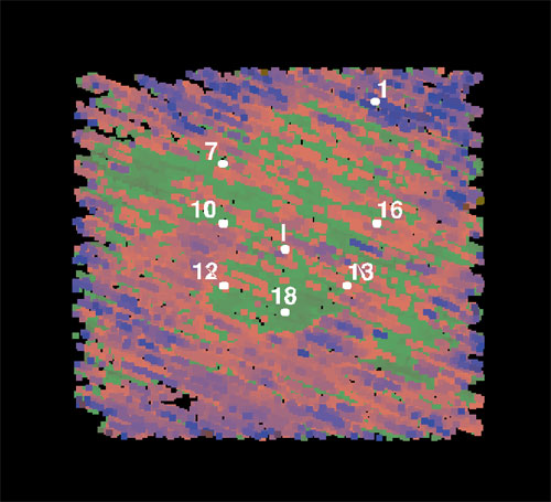
Figure 6A--Baseline Survey-Color representation of instantaneous frequency for a 24 msec-thick slice at a depth of around 560 msec for the baseline 3-D survey conducted when the field was fully pressurized with water and just prior to the first injection of CO2. A larger version of this figure is available.
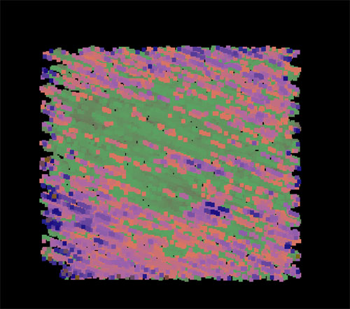
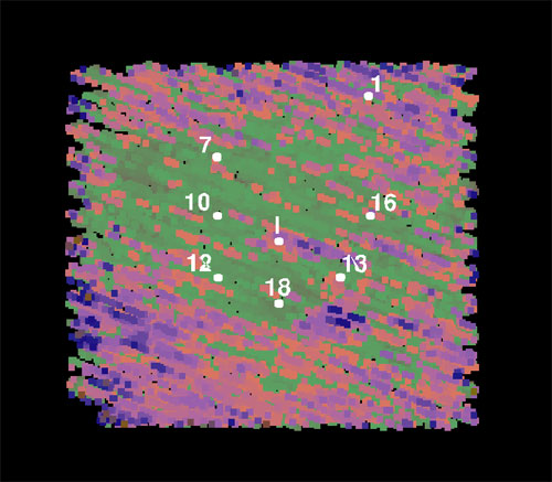
Figure 6B--Same plot with wells located. Well locations (coordinates based on conversions from legal descriptions) are placed to improve spatial awareness of the key locations around the field. A larger version of this figure is available.
An obvious northwest to southeast grain is evident in the IF plots. This grain is the result of rotating the grid 120° during processing to improve the distribution of subsurface samples. Values in each cell are independently calculated from CMP traces within that cell only and are in no way influenced by CMP traces gathered within adjoining cells. Therefore, the discrete, blocky character of the displayed data is a result of the receiver line orientation (trends along inline direction) and rotation of the seismic bins.
Some sense of the lithologic trends potentially influencing the performance observed at the various wells can be gained by comparing and contrasting apparent boundaries and changes to the texture of specific seismic properties across the site. In making these observations keep in mind that both the amplitude and frequency attribute plots (Figure 7) show response changes for seismic volumes representing an interval of rock over 100 ft thick that includes the subsurface interval of interest. Thus some of the data characteristics observed may be from overlying and underlying beds or changes in the "C" zone may be subdued by consistent seismic response from overlying and underlying beds. A prominent feature evident in both plots is a contrast in properties north and south of an east/west trending line (A) lying immediately south of well #18 (Figure 7). This trend (A) marks a substantial change in seismic character on both amplitude and frequency plots and may indicate the presence of a structural feature or an abrupt change in rock properties. Another lineament (B) follows a high (red) trend on the amplitude plot and an anomalous group of cells on the frequency plot. This feature, though subtle on both plots, is interpreted to exhibit sufficiently high contrast to represent a marked change in rock properties of some kind. A third more subtle northeast/southwest trending lineament (C) marks a change in texture on the frequency plot and an apparent alignment of anomalies on the amplitude plot. Because of the greater sensitivity of instantaneous frequency to lateral lithologic changes in comparison with instantaneous amplitude, it seems likely this (C) lineament may be related to a lithologic change. It is unlikely the (C) lineament would have been interpreted from amplitude plots alone. The lineament features are consistent with pressure and modeling data and models of the pilot.
Figure 7A--Baseline Survey-Lineaments based on changes in data character or texture were interpreted on baseline data from 24 msec time slices at around 560 msec. These lineaments are interpreted identically on both displays--instantaneous frequency (7A) and amplitude (7B). A larger version of this figure is available.
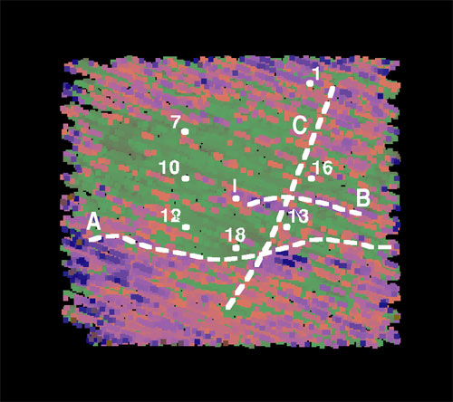
Figure 7B--Color representation of amplitude values along the 560 msec time slice with lineaments displayed. A larger version of this figure is available.
Analysis and comparison of the baseline and first and second monitoring surveys show changes in instantaneous frequency within the study area (Figures 6, 8, and 9). Because of the thickness of the seismic volume, equalization, and IF response issues, interpreting these data at this stage will be limited to identification of areas where changes occur between surveys. All significant changes observed in these data are generally within an area defined by wells number 12, 18, 13, 16, 7, 10, and 1 (Figure 10B). Comparing and contrasting the two monitor surveys with the baseline survey, changes in IF can generally be grouped in one of four ways: 1) similar change in both monitoring surveys, 2) change in the first survey not evident on the second survey, 3) change in the first survey and a different change in the second survey, and 4) no change in the first survey but change in the second survey. The third monitoring survey obtained June 23-July 1 will provide a further examination of the consistency of changes in different areas. Definition of the LKC "C" zone wavelet will also refine changes.
Figure 8A--First Monitoring Survey--Instantaneous frequency plots of the first monitor survey using an identical color scale as used on the baseline. A larger version of this figure is available.
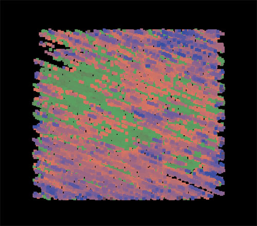
Figure 8B--Well locations are estimated from conversion of legal descriptions, so some inaccuracy exists in their locations. A larger version of this figure is available.
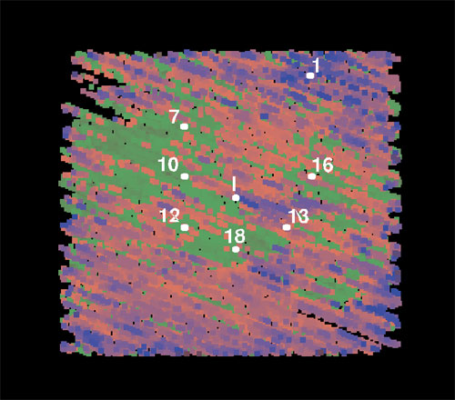
Figure 9A--Second Monitoring Survey--Instantaneous frequency plots of the same 24 msec time slice as displayed for monitor survey one and the baseline survey. Color scales and well locations are identical for all IF plots. A larger version of this figure is available.
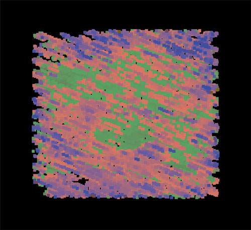
Figure 9B--Well locations are estimated from conversion of legal descriptions, so some inaccuracy exists in their locations. A larger version of this figure is available.
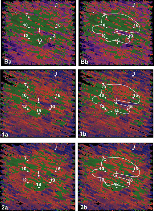
The evident changes in texture for the general CO2 pilot region compared to outside the flood region lend support to the idea that changes are being detected. However, interpretation of the causes for the differences observed between the monitor surveys is not yet clear nor is the size of the area of change in the subsurface compared to the seismic response fully resolved (Figure 10). Volumetric analysis precludes the possibility that change observed in the entire region shown in Figure 10 represents significant CO2 invasion. Assuming CO2 was flooding only a 1-foot thick interval with the CO2 displacing only 25-33% of the oil/water in the pores at pressures ranging radially away from the well from 1,800 to 700 psi, it is possible that the change observed only in the northeastern quarter could be due to CO2 invasion at the time of the first monitor survey (Figure 10 Bb). However, this would require that CO2 moved along a focused region or arc and did not move radially out into the formation from the CO2I#1. Insufficient CO2 volume was injected at the time of the first monitor survey to affect the entire area simultaneously. However, seismic response will noticeably change with a small percentage change in saturation of CO2. As well, considering the size of the Fresnel zone, "fingering" will appear enlarged on seismic data. Depending on the geometry of the "fingering," seismic images could easily represent thin, zone of higher CO2 saturation that are moving through the reservoir.
Figure 10--Comparison of baseline (B), monitor 1 (1), and monitor 2 (2) IF plots with wells located (a). The area highlighted possessed notable changes in data character, intensity, and/or texture between the three surveys. Changes between surveys are not necessary consistent due to a variety of reasons (equalization, changes in reservoir, etc.), but the changes observed within the highlighted area seem to suggest that as the CO2 has progressed the subsurface in proximity to the injector is experiencing changes. A larger version of this figure is available.
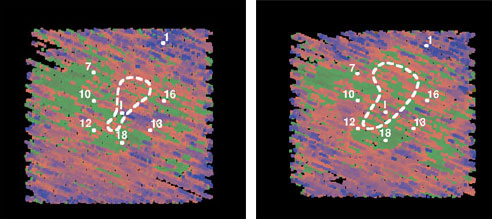
In general changes on the monitor surveys relative to the baseline survey are predominantly north of CO2I#1 (Figure 11). Changes are evident south of CO2I#1 but they appear less coherent as a mass and seem to generally increase in areal extent on the second survey relative to the first. When considering the extremely small percentage change expected in seismic properties of the L-KC "C" for this study, changes from one monitor survey to the next on these particular preliminary analyses might not be numerically consistent. Areas consistently changing rather than consistent change relative to the baseline survey are the targets of the seismic attribute analysis at this point in the interpretations. Between Monitoring Surveys One and Two, injection in CO2#10 was increased which might have resulted in a change in fluid saturation distribution. Analysis of survey results with field pressure, injection, and production data is being performed for integrated interpretation.
Figure 11--Monitor survey one (on left) and monitor survey two (on right) with the areas possessing the greatest and most consistent change relative to the baseline survey outlined with a dashed line. These areas of greatest change are not necessary numerically consistent with each other, but they do, from a relative perspective, contain the set of cells that define the greatest overall relative change. A larger version of this figure is available.
With initial CO2 detected in Colliver #12 near the end of May, this third monitor survey provides an important snapshot for reconstructing the time-lapse path CO2 has taken moving through the field from injector to producer. Based on pre-injection models, progression of CO2 from injector to producers as well as the volumetric expansion of the CO2 slug was expected to preferentially move toward Colliver #12.
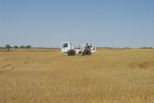
This third survey was delayed a few weeks until after wheat harvest, avoiding significant damage to the wheat crop being grown on about one-third of the survey area. On June 25 the last of the wheat still standing within the patch was harvested. An unusually rainy June also played a role in delaying acquisition by several days. Ground conditions were ideal for receiver coupling immediately after harvest with only stubble left in the fields (noise from wheat moving with the wind was all but eliminated) and because of the 3+ inches of rain that fell the week prior to the start of this third monitor survey (Figure 12). A negative aspect of these ideal receiver conditions was the softer than previous ground conditions, which with a vibrator source reduces the efficiency of the energy transfer process.
Figure 12--View looking west showing vibrator sweeping in the wheat stubble field surrounding the CO2 injection well. Colliver #12 is visible on the horizon to the left of the vibrator in this picture. The CO2 injector is enclosed in a yellow steel protection fence and can be seen immediately behind the vibrator, in the distance. Combines completed cutting wheat from this field just days before this picture was taken.
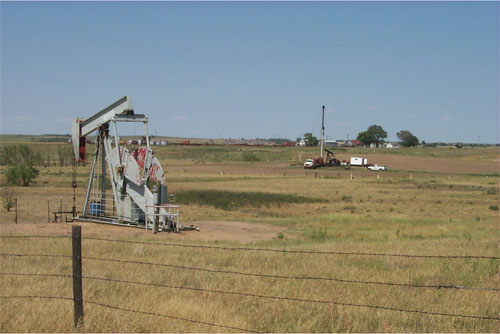
Surface conditions changed between the end of March and end of June surveys. Geophone planting conditions were very similar while surface activity and associated noise was quite different. Noise from cattle and farm equipment provided new challenges to data acquisition and processing. Cattle were penned away from the receiver lines but were still were close enough to be a source of noise on the northernmost receiver line (Figure 13A). This third monitor survey was scheduled as soon as possible after the second monitor survey while avoiding wheat harvest, rain, and the plugging of Colliver #2 (Figure 13B).
Figure 13 Noise sources and unique acquisition obstacles change with each survey and the seasons. 13A--Cattle in the pasture immediately north of the CO2 injector.
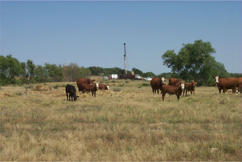
Figure 13B--Colliver #7 pumping in the foreground and Colliver #2 being plugged in the background.
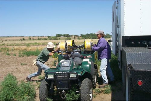
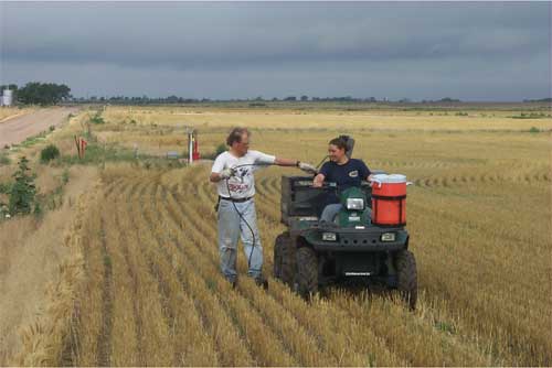
Ground and weather conditions were ideal during the first several days of acquisition. With over 3 inches of rain falling days prior to the deployment of receivers, planting and coupling conditions were very good and better than expected for this area during this time of the year (Figure 14A). Geophone locations were DGPS surveyed to be within a few centimeters of previous geophone locations. Because the wheat had just been harvested the cables could be laid quickly through the stubble with ATVs, reducing the extra care necessary on previous surveys to minimize damage to growing crops (Figure 14B).
Figure 14A--Geophones were planted in a 0.3 m equilateral triangle centered on the DGPS-located station.
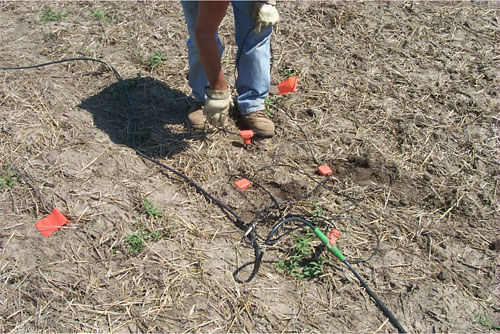
Figure 14B--Weatherproofed re-enforced Ethernet cables stored on spools connected the eleven 24-channel Geometrics Geodes to the NZC seismic controller. These cables were deployed using a custom cable handling system.
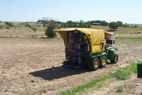
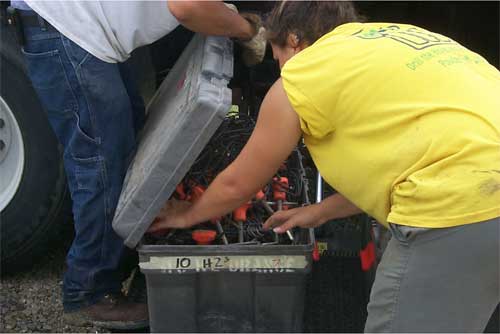
Two 24-channel Geodes were deployed in the center of each receiver line (Figure 15A). These 24-bit A/D distributed seismographs transmit their digital data through four unique Ethernet lines daisy chained between units located at the center of each of the five receiver lines. An 85-amp-hour deep-cycle marine 12-volt battery powered two units for more than 40 hours of continuous use. The four Ethernet lines were all connected to the NZC controller located centrally within the receiver patch (Figure 15B). Warm and clear weather conditions allowed open-air operation of the seismic controller. Temperatures ranged from lows of 60° F to highs near 90° F.
Figure 15A--One of five Geode deployments located in the center of each 48-station receiver line.
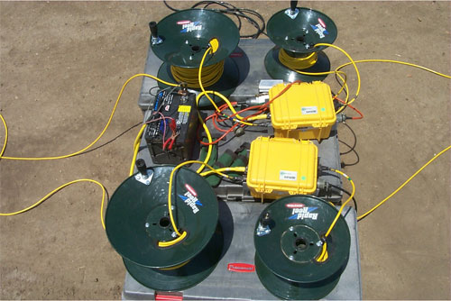
Figure 15B--The five Geode groupings were all connect the Geometrics StrataVisor NZC seismic controller. Operated from this John Deere Gator, seismic operations were all-weather and all-terrain. Here the Gator is configured for warm dry conditions. Under wet or cold conditions an additional zip-on covering can be added to protect the operator and seismographs.
Shot gathers from this survey were of similar quality to those from the previous three surveys (Figure 16). Wind was light and variable with speeds not exceeding 15 mph. Noise from the fixed sources (pump jacks, pipelines, and power lines) is evident as on previous surveys. Vehicle noise on county roads was random, but was overall equivalent in volume and frequency to previous surveys as well. Unique to this survey was the noise from cattle movement near line 1 and the combine harvesting wheat on June 25 near the east end of lines 3 and 4. Contributions by both these noise sources, new to this third monitor survey, were minimized due to their non-stationary nature and the collection of four-sweep vertical stacks at each station.
Figure 16-A single sweep from near center of the receiver spread. This shot gather has been scaled to enhance reflections within the 2500 to 3500 ft depth range. Reflections from the L-KC "C" zone will arrive between 550 and 650 msec across this spread. This range of arrival times is directly related to source-to-receiver offset and associated non-linear increase in travel path with source-to-receiver separation. A larger version of this figure is available.
An apparent dominant frequency of around 120 Hz at 1,000 ft and 60 Hz at 3,000 ft will be increased by 50% at 1,000 ft and doubled at 3,000 ft during processing using spectral balancing techniques (band-limited spiking deconvolution). Vibrator ground force was around 12,000 lb at 60 Hz, decreasing linearly to around 6,000 lbs at 200 Hz. Spectral properties of the recorded data are controlled by the source energy spectrum (power as a function of frequency) and the natural attenuation of higher frequencies by the earth. With large dynamic range recording systems and minimal background noise, low amplitude signal at higher frequencies can be enhanced to some degree relative to the more dominant lower frequency recorded energy.
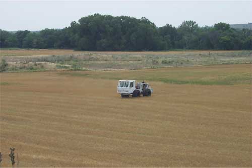
Data quality on this fourth survey (third monitor survey) is not quite as high as on the previous two monitor surveys. Considering the efforts taken to insure exact duplication in equipment and parameters, this difference is clearly related to the ability of the ground surface to accept and propagate seismic energy (Figure 17). The noticeable enhancement in coupling between receivers and the ground was likely due to the substantial rainfall that preceded the survey. Unfortunately the softer ground conditions that resulted from the rain adversely affected energy transmission by the source into the ground. Ground force curves, as calculated using the baseplate and mass accelerometers, were consistent with previous surveys, while the recorded energy levels at the receivers were down. The difference is clearly related to the saturated nature of the upper 1 ft of soil in this area.
Figure 17A--November 2003 survey.
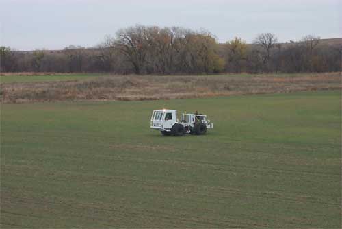
Figure 17B--January 2004 survey.
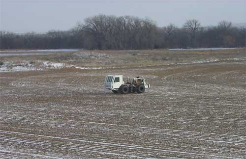
Figure 17C--March 2004 survey.
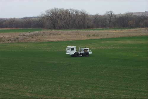
Figure 17D--June 2004 survey (lower right).
Data acquisition for this third monitor survey required eight days to complete with an additional two days of land surveying to relocate receiver stations after wheat harvest was completed and cattle were put out to graze across part of the survey area. An additional day of surveying was necessary to exactly locate the wells within the survey grid. With another almost 2 inches of rain falling the night after the final sweeps were recorded for this survey, small footprint, low ground pressure vehicles really saved the day in keeping the equipment free of excessive mud and avoiding damage to farm fields and pastures (Figure 18). Equipment was picked up and the site secured in a day.
Figure 18A and B--With almost 2 inches of rain the night after acquisition was complete, the six-wheel drive ATVs were instrumental in picking up and transporting cables and phones back to the semi-trucks where they were loaded for transport back to Lawrence without "rutting" the farmer's fields and pastures.
With the unusually large amounts of June rainfall most flowering plants and grasses were quite lush (Figures 19 and 20). Vegetation had not yet reach full growth, so moving along the lines with the vibrator and obtaining good source pad coupling were not impaired by excessive organic materials.
Figure 19A--Sunflower blooming during this late June survey.
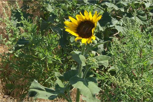
Figure 19A--Thistle blooming during this late June survey.
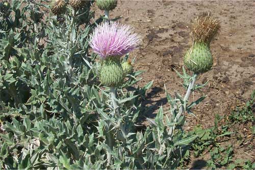
Figure 20--View looking west near #8 (first image). Heavier vegetation than on previous surveys did not result in a noticeable increase in noise or access problems.
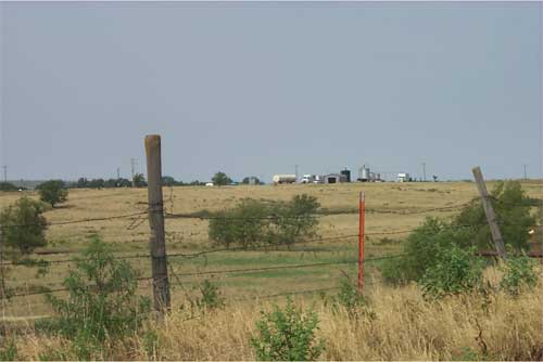
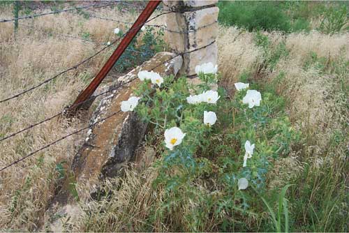
Figure 21--On several occasions local residents were the source of unusual noise bursts on recorded data. Arrival of a crewmember to investigate was usually sufficient to discourage these critters from hanging around the seismic line.
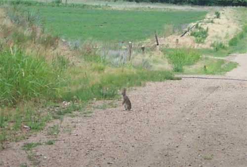
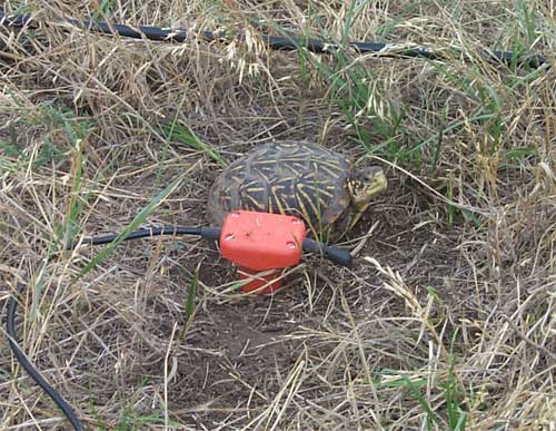
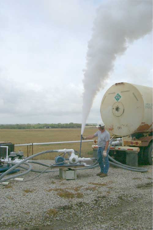
Figure 22--Kevin Axelson, Murfin production foreman, vents CO2 after the installation of a new pump.
|
Kansas Geological Survey, 4-D Seismic Monitoring of CO2 Injection Project Placed online July 22, 2004 Comments to webadmin@kgs.ku.edu The URL is HTTP://www.kgs.ku.edu/Geophysics/4Dseismic/Reports/Jun23_2004/index.html |