![]()
Prev Page--Formations || Next Page--Conclusions
Hydrology
Hydrologic Properties of Water-Bearing Materials
The quantity of ground water that an aquifer will yield to wells depends upon the hydrologic properties of the aquifer. The ability of an aquifer to transmit water is measured by its coefficient of transmissibility. The coefficient of transmissibility (T) of an aquifer is defined as the number of gallons of water that will move in 1 day through a vertical strip of aquifer 1 foot wide and the full thickness of the aquifer, under a hydraulic gradient of 100 percent, or 1 foot per foot, at the prevailing temperature of the water. The coefficient of permeability (P) is expressed as the rate of flow of water, in gallons per day, through a cross-sectional area of 1 square foot under a hydraulic gradient of 1 foot per foot. The coefficient of permeability can be computed by dividing the coefficient of transmissibility by the thickness (m) of the aquifer. The coefficient of storage (S) of an aquifer is defined as the volume of water it releases or takes into storage per unit surface area of the aquifer per unit change in the component of head normal to that surface. Under water-table conditions the coefficient of storage is practically equal to the specific yield, which is defined as the ratio of the volume of water a saturated material will yield to gravity in proportion to its own volume.
Purpose of Aquifer Tests
The hydrologic properties described above are determined from aquifer tests. Hydrologic coefficients resulting from aquifer tests are used in conjunction with the water-level contour maps to estimate the quantity of ground water moving laterally through the water-bearing formations. They are used to estimate the quantity of water being removed or returned to storage and the amount of local recharge. These tests also give an indication of the type and areal extent of the water-bearing materials.
Methods of Analyses and Test Results
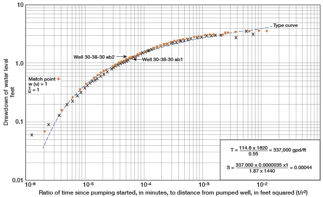
Aquifer tests were made at 26 sites in Grant and Stanton counties. The tests were analyzed by the nonequilibrium method (Theis, 1935) or by the modified nonequilibrium method (Cooper and Jacob, 1946). These methods of analyses are also shown in U.S.G.S. WSP1536-E. The results of these tests are summarized in Table 5. The basic data for one of these tests are plotted in Figure 6. The coefficients of transmissibility obtained from these tests are plotted on Plate 11B in parentheses to distinguish them from the estimated coefficients to be described later.
Table 5--Results of aquifer tests, Grant and Stanton counties.
| Well number | Geologic source (a) |
Coefficient of transmissibility, gpd/ft |
Coefficient of storage, dimensionless |
|---|---|---|---|
| Grant County | |||
| 27-36-15dd | Npl, No | 153,000 | 0.00014 |
| 27-37-29cc | Npl, No | 52,100 | .00012 (b) |
| 27-38-15da | Npl, No | 63,400 | .00023 (b) |
| 27-38-19cd | Npl, No | 590,000 | .0048 |
| 27-38-22cb | Npl, No | 159,000 | .00035 |
| 27-38-23ca | Npl, No | 71,000 | .00021 |
| 27-38-32bb | Npl, No | 188,000 | .0024 |
| 28-36-11ba | Npl, No | 215,000 | .00022 |
| 28-38-12cb | Npl, No | 50,600 | .00028 |
| 28-38-15cb | Npl, No | 119,000 | .00060 |
| 28-38-27ba | Npl, No | 125,000 | .00021 |
| 29-35-15ab | Npl | 134,000 | .00038 (b) |
| 29-38-35db | Npl, No | 45,000 | .00094 (b) |
| 30-37-2ba2 | Npl, No | 29,600 | .00014 (b) |
| 30-37-19aa2 | Npl | 56,000 | .00029 (b) |
| 30-37-26da | Npl, No | 145,000 | .0032 |
| 30-38-30ac | Npl, No | 337,000 | .00044 (c) |
| Stanton County | |||
| 27-39-13ac | Kd, Kc | 45,800 | |
| 27-40-25cb | Npl, No | 137,000 | .0048 |
| 28-39-12ac | Npl | 40,500 | .00011 |
| 28-39-20bd | Npl, No | 188,000 | .00095 |
| 28-39-24cc2 | Npl, No | 465,000 | .0094 |
| 28-41-14aa | Npl, No | 352,000 | .059 |
| 29-39-24dd | Npl, No | 58,000 | .0011 (b) |
| 30-40-24cd | Npl, No, Kd | 97,500 | .0013 |
| 30-41-13cc | No, Kd | 137,000 | .044 |
| a. Npl, Pleistocene deposits; No, Ogallala Formation; Kd, Dakota Formation; Ke, Cheyenne Sandstone. |
|||
| b. Pumped well may be partially penetrating. | |||
| c. See Figure 7. | |||
Figure 6--Drawdown of water level in observation wells during 30-38-30ac aquifer test, July 27-31, 1960.
The values for T obtained from these tests were reduced to the field coefficients of permeability (P - T/m). The value used for m is not the total saturated thickness of the formations, but is the aggregate of effective thickness of the sand and gravel beds in the formation, based on the driller's and authors' interpretations of the well logs.
Because tests were made using wells screened opposite more than one aquifer, a trial and error method was used to determine P for each aquifer. Trial values of P were assigned to the sand of each aquifer, then multiplied by the aggregate thickness to obtain T. A trial T for the complete saturated sand section was then obtained by adding the individual values for T for each aquifer. This value for T was then compared with that obtained from the aquifer test. The process was continued until a permeability (P) was assigned to each aquifer that when combined with the aggregate thickness of the aquifers at each test site resulted in coefficients of transmissibility that were approximately the same as the coefficients obtained from aquifer tests. Using this method, the average coefficient of permeability was 2,200 gpd/ft2 for the Pleistocene aquifer and 1,250 gpd/ft2 for the Pliocene aquifer.
The coefficients (P) were then extended to other areas and used in conjunction with the drillers' logs to estimate the coefficients (T) as shown for well 27-35-4bbb. In this well there is a saturated section of 112 feet of sand and/or gravel in the Pleistocene deposits and 33 feet of Pliocene sand. Thus: (112 X 2,200) + (33 X 1,250) = 287,000 gpd/ft which is the coefficient (T) for the well site. The estimated transmissibilities obtained by this method are shown in brackets on Plate 11B.
The thickness of the sand and gravel used in the above estimates is not the total thickness of sand and gravel in the well described by the drillers. In many of the logs, the drillers, on the basis of their experience, assigned a yield number to each sand and gravel section of the aquifer. If a 10-foot section of aquifer contained clean sand and gravel and the material drilled easily, the driller probably would assign it a thickness of 10 feet. However, if the 10-foot section contained thin layers of silt or fine sand, the driller might assign it a thickness of 5 feet. In other words, the numbers shown in parentheses on the drillers' logs are the drillers' estimates of the yield from the intervals logged. The drillers total these numbers for the well and multiply by a coefficient to obtain the estimated yield of a well in gallons per minute. Where these estimates were not included in the drillers' logs, the equivalent thicknesses were estimated by the authors. The estimates of the authors were not included in the published logs but are computed as part of the coefficients of transmissibility on Plate 11B.
Because of the reasons discussed on page 49 of this report, the coefficients of storage obtained from the foregoing tests were not used in the quantitative computations. However, the coefficients did indicate that artesian conditions existed during the pumping tests.
Water Levels
History of Water Levels
Very little is known about the water levels in the area prior to 1940. During the field work in the early 1940's, observation wells, were established in the area, and periodic measurements have been made since that time. As shown by the hydrographs (Fig. 7), the water levels remained approximately at the same level or trended slightly upward through the period 1940-52, then declined at a slow rate. After 1952, the effect of pumping for irrigation is reflected on the hydrographs and masks the effect of precipitation in the area.
Figure 7--Hydrographs of wells in the Grant-Stanton area.
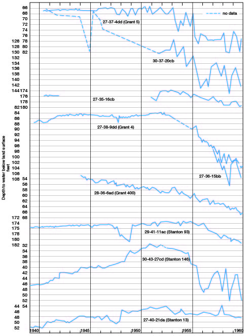
Most of the water levels measured during and since 1957 have been in irrigation wells that obtain water from unconsolidated aquifers. These are gravel-walled wells which are perforated opposite all water-bearing materials penetrated in the well. Thus, these measurements are of the composite water levels for all the formations penetrated in each well (Tables 16, 17, 18).
Few wells in the area are perforated only in the sandstone aquifers. A few scattered wells were perforated both in the unconsolidated and the sandstone aquifers to the bottom of the Cheyenne Sandstone. The water levels in these wells, cased through the sandstone aquifers including the Cheyenne Sandstone, were compared with water levels in nearby wells screened only in the unconsolidated materials. The water levels in these two types of wells were at approximately the same level; hence, it was assumed that the 1960 water levels throughout the area were at approximately the same level in wells screened in both the unconsolidated and consolidated aquifers throughout the Cheyenne Sandstone. Little is known about the water levels in the Triassic sandstone, but they probably are comparable with those in the unconsolidated aquifers of the area. However, in northeastern Grant County, the flow in the Triassic sandstones is probably toward the east or northeast as compared with the southeasterly flow in the unconsolidated materials, and there may be some difference in water levels in this area.
During most years, pumping for irrigation causes considerable decline of water levels during the summer months, but some recovery of water levels is noted during the late winter and early spring months. An example of this is shown by fluctuations in well 28-38-8bc. Water levels in this well were as follows: during the late summer of 1959, 180 feet reported; March 21, 1960, 79.7 feet; and January 22, 1963, 110 feet. Pumping for irrigation in 1959 was mostly during the summer months, but in 1962, pumping was continued through December in addition to the summer months. The above well was not measured in 1962, but fluctuations in well 28-38-27ca can be used as an example. Water levels in this well were: March 30, 1960, 81.7 feet; Sept. 6, 1962, 150.7 feet; Oct. 11, 1962, 138.5 feet; Nov. 1, 1962, 123.6 feet; and Jan. 22, 1963, 103.7 feet.
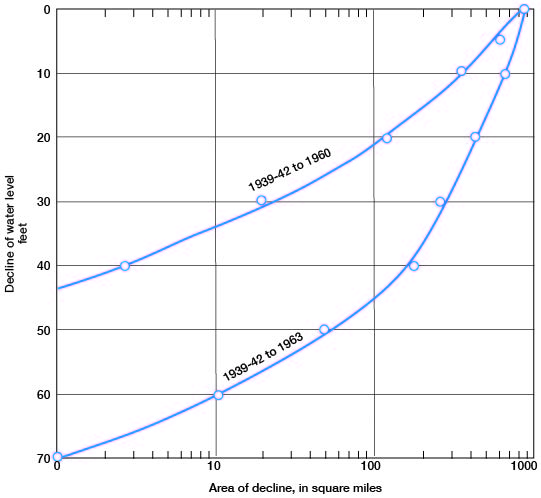
Figure 8--Decline of water level in in the Grant-Stanton area.
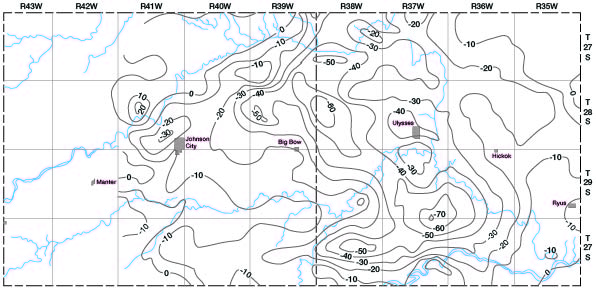
The change in water levels in much of Grant and Stanton counties from about 1940 to Jan. 22, 1963, is shown in Figure 9. Figure 9 was prepared from Plate 11A which shows the water level as of 1939-42 and from an unpublished map which shows the water level for Jan. 22, 1963. Plate 11A was superimposed over the 1963 map and contours drawn through points of equal change. A map showing the change from about 1939-42 to March-April 1960 was given by Broeker and Fishel (1962, p. 31). If Figure 9 is compared with the acreage irrigated (Pl. 12), the close correlation between decline in water level and the areal distribution of pumping for irrigation may be noted.
Figure 9--Change of water level in Grant and Stanton counties from 1939-42 to January 22, 1963. A larger version of this figure is available.
The areal decline of water level from 1939-42 to 1960 and from 1939-42 to 1963 is shown graphically in Figure 8. The water level declined (1939-42 to 1963) 70 feet or more in an area of less than 1 square mile, 60 feet or more in 10 square miles, 40 feet or more in 174 square miles, 20 feet or more in 420 square miles, and 10 feet or more in 662 square miles.
Withdrawals of Ground Water
by Carl E. Nuzman, Engineer,
Division of Water Resources,
Kansas State Board of Agriculture
The Geological Surveys' open file well records first reported the use of wells for irrigation in this area in 1940. As of that date, there were 4 irrigation wells in Stanton County and 8 in Grant County. The publication, "United States Census of Irrigation--Kansas 1940," listed 319 acres irrigated in Stanton County but did not mention Grant County. A report to the Governor of Kansas in 1944 listed 330 acres irrigated in Stanton County and 1,178 acres in Grant County. A report for 1948 by the Extension Service of Kansas State University listed 7,520 acres irrigated in Stanton County and 12,500 acres irrigated in Grant County. The Kansas Water Resources Board furnished reports of water usage for the period 1950 through 1957. The withdrawals for 1958 through 1960 (Table 6, 7) are compilations of the data furnished directly to the Division of Water Resources. In 1960 an estimated 68,000 acres were irrigated in Stanton County and 81,000 acres were irrigated in Grant County. The information obtained from the above sources is summarized in Figure 10, which demonstrates the growth of irrigation in the area.
An examination of the records indicates that in 1960 less than 4,000 acre-feet per year was pumped for municipal, rural, and industrial use. As this is less than 2 percent of the total use, or within the limit of error in estimation of irrigation use, only the irrigation use is shown in Figure 10 and Tables 6 and 7.
Table 6--Reported pumpage from irrigation wells (acre-feet) in Grant County, 1958-1960
| Well number | 1958 | 1959 | 1960 |
|---|---|---|---|
| 27-35-10cc | 640 | 674 | 616 |
| 27-35-17ad | 810 | 432 | |
| 27-35-24ac | 1,406 | ||
| 27-35-27ca | 1,810 | 2,570 | 1,175 |
| 27-35-29ba | 865 | 788 | |
| 27-35-33bb | 880 | 344 | |
| 27-36-13ad | 804 | 240 | |
| 27-36-14cc | 1,369 | ||
| 27-36-15dd | |||
| 27-36-15cc | 997 | 1,148 | |
| 27-36-18dc | 636 | 436 | 532 |
| 27-36-21dc | |||
| 27-36-23dc | |||
| 27-36-25aa | 716 | ||
| 27-36-25cc | 517 | 716 | |
| 27-37-3bd | |||
| 27-37-3dd | |||
| 27-37-4ab | |||
| 27-37-11ab | 352 | 344 | |
| 27-37-14ba | 1,044 | 625 | |
| 27-37-16bb | 141 | 409 | 380 |
| 27-37-19db | 716 | 1,363 | |
| 27-37-20cd | 684 | 1,249 | 1,326 |
| 27-37-25cb | 811 | 402 | 459 |
| 27-37-26bc | 392 | 1,231 | 1,194 |
| 27-37-28cb | 186 | ||
| 27-37-29cb | |||
| 27-37-29cc | 772 | 1,190 | 1,274 |
| 27-37-30bd | 681 | 955 | 1,243 |
| 27-37-33cc | 263 | 394 | 398 |
| 27-37-34bc1 | |||
| 27-37-34da | 257 | 292 | 454 |
| 27-37-35dc | 456 | 168 | |
| 27-37-36cc | 302 | ||
| 27-38-1da | 106 | 354 | |
| 27-38-6cb | 320 | ||
| 27-38-12ad | |||
| 27-38-12dd | 361 | 276 | |
| 27-38-13ab | 299 | 229 | |
| 27-38-13cc | 157 | 155 | 158 |
| 27-38-14cd | 99 | 238 | 265 |
| 27-38-15bb | 252 | 241 | 253 |
| 27-38-15da | 88 | 292 | 353 |
| 27-38-19bc | 270 | 967 | |
| 27-38-19db | 112 | ||
| 27-38-20bd | 333 | ||
| 27-38-20cb | 219 | ||
| 27-38-21cb | |||
| 27-38-22cb | 860 | 661 | |
| 27-38-22cc | 859 | 1,115 | |
| 27-38-23ca | 717 | 728 | |
| 27-38-23cb2 | 587 | 317 | |
| 27-38-24cc | 532 | 666 | |
| 27-38-25bb | |||
| 27-38-26bb | 367 | 516 | 545 |
| 27-38-27aa | 1,032 | ||
| 27-38-27bb | 251 | 332 | |
| 27-38-28cb3 | 709 | 1,216 | 927 |
| 27-38-29ac | 1,080 | 1,524 | |
| 27-38-30ca | 875 | 1,105 | |
| 27-38-30cb | 825 | ||
| 27-38-31ba | 516 | ||
| 27-38-31dd2 | 826 | 1,261 | |
| 27-38-32bb | 1,524 | ||
| 27-38-32bc | |||
| 27-38-32cc | 405 | 545 | |
| 27-38-33cb | |||
| 28-35-5bc | 566 | ||
| 28-35-5dc | 666 | 662 | |
| 28-35-6ba | 1,420 | 1,199 | 1,192 |
| 28-35-8bb | 1,335 | ||
| 28-35-9aa | 994 | 1,290 | 551 |
| 28-35-10bb | 182 | ||
| 28-35-15cb | 267 | 305 | |
| 28-35-20ab | 870 | 985 | 905 |
| 28-35-21bb | 445 | 691 | 395 |
| 28-35-22ac | 336 | 258 | |
| 28-35-22bb | 363 | 398 | 407 |
| 28-35-23bd | 325 | ||
| 28-35-27bb | |||
| 28-35-27bc | 940 | ||
| 28-35-29bc | 1,326 | 1,237 | |
| 28-35-30bb | 811 | 624 | |
| 28-35-31cd1 | 5 | ||
| 28-35-31cd2 | 61 | ||
| 28-35-35dc | 994 | 690 | |
| 28-35-36ab | 476 | 649 | 759 |
| 28-36-2ba | 420 | 492 | |
| 28-36-2cd | 420 | ||
| 28-36-11ba | 625 | 1,095 | |
| 28-36-13ac | 254 | 744 | 423 |
| 28-37-2bb | 182 | ||
| 28-37-2bc | 177 | ||
| 28-37-4ac | 122 | 269 | 244 |
| 28-37-6bb | 374 | 239 | |
| 28-37-7cb | 134 | 428 | 530 |
| 28-37-9ac | |||
| 28-37-9bb | 363 | 444 | 613 |
| 28-37-9cc | 272 | 431 | |
| 28-37-10bc | 412 | ||
| 28-37-17cb | 848 | ||
| 28-37-20cd2 | 530 | ||
| 28-37-22ab | 177 | ||
| 28-37-27cc1 | |||
| 28-37-27cc2 | 158 | ||
| 28-37-27cd | 490 | ||
| 28-37-28dc | 500 | 398 | 276 |
| 28-37-28dd1 | 200 | 155 | 94 |
| 28-37-28dd2 | 500 | 471 | 446 |
| 28-37-30bb | 923 | 1,147 | |
| 28-37-31aa1 | |||
| 28-37-31aa2 | 107 | 107 | |
| 28-38-4bb | 293 | ||
| 28-38-4cc | 420 | ||
| 28-38-5ac | 536 | ||
| 28-38-5bd | 658 | 1,946 | |
| 28-28-5dc | 1,400 | 420 | |
| 28-38-6bc | |||
| 28-38-6cb | |||
| 28-38-7ab | 321 | 243 | |
| 28-38-7bb | |||
| 28-38-8bb2 | 1,236 | 1,503 | 1,095 |
| 28-38-8bc | 348 | 265 | 203 |
| 28-38-9ca | 795 | 1,105 | 1,050 |
| 28-38-9cb | 6 | 7 | |
| 28-38-10ab | |||
| 28-38-10bb | 1,247 | ||
| 28-38-12bc | |||
| 28-38-12cb | 308 | 864 | 1,166 |
| 28-38-15cb | |||
| 28-38-16ab | |||
| 28-38-16bb | 928 | 176 | |
| 28-38-16cb | 407 | ||
| 28-38-16db1 | 231 | ||
| 28-38-16db3 | |||
| 28-38-17ab | 828 | 1,574 | |
| 28-38-17bb | 608 | 1,193 | |
| 28-38-17cb | 862 | 1,432 | |
| 28-38-18bb | 1,079 | 1,538 | 1,263 |
| 28-38-18db | |||
| 28-38-18dc | 309 | 795 | |
| 28-38-19bc | 862 | 1,314 | 888 |
| 28-38-19bd | 994 | 726 | 650 |
| 28-38-20dc1 | 495 | 840 | 322 |
| 28-38-20dc2 | 435 | 371 | |
| 28-38-27ba | |||
| 28-38-27ca | 1,784 | 958 | |
| 28-38-27cb | |||
| 28-38-28da | 1,200 | 1,505 | |
| 28-38-30cb | 640 | 159 | |
| 28-38-30cc | 482 | ||
| 28-38-31db | 786 | 628 | |
| 28-38-33ba2 | |||
| 28-38-33bd | |||
| 28-38-35bc | 663 | 942 | |
| 29-35-6ba | 490 | 582 | |
| 29-35-7bc1 | |||
| 29-35-7bc2 | |||
| 29-35-7cb1 | |||
| 29-35-7cb2 | 422 | ||
| 29-35-12dd | 130 | 141 | |
| 29-35-13ac | 868 | 835 | |
| 29-35-15ab | 561 | ||
| 29-35-24ba | 817 | ||
| 29-35-24bc | 2,298 | 1,390 | |
| 29-35-25dc1 | |||
| 29-35-25dc2 | |||
| 29-35-25dc3 | |||
| 29-35-25dd2 | |||
| 29-35-25dd3 | 101 | ||
| 29-36-19bc | |||
| 29-36-30bc | 62 | ||
| 29-36-30dc | |||
| 29-36-31db | 269 | 221 | 316 |
| 29-37-8cb | 362 | 636 | |
| 29-37-19db | 1,031 | 550 | |
| 29-37-21bc | 998 | ||
| 29-37-22aa | |||
| 29-37-22cc2 | 610 | 949 | 486 |
| 29-37-26cc | 823 | ||
| 29-37-28bb | 132 | 707 | 321 |
| 29-37-28cb | 919 | 687 | |
| 29-37-29bb | 561 | 497 | |
| 29-37-32bd | 577 | 450 | |
| 29-37-32cc1 | 364 | ||
| 29-37-32db | 390 | ||
| 29-37-34bd | 486 | 318 | |
| 29-37-35ac | |||
| 29-37-35cc | 566 | ||
| 29-37-35cd | |||
| 29-38-1bb | 790 | 954 | |
| 29-38-1ca | 530 | ||
| 29-38-3ba | 960 | 1,467 | |
| 29-38-4cc | 531 | 550 | |
| 29-38-5aab | |||
| 29-38-5aac | 406 | 403 | 430 |
| 29-38-7da | 1,114 | 1,230 | |
| 29-38-8cc | 1,127 | 921 | |
| 29-38-22bb | 344 | 440 | |
| 20-38-22cb | 728 | 808 | 529 |
| 29-38-25ba | 367 | 171 | 330 |
| -99-38-27ad | 380 | 456 | 474 |
| 29-38-31dc | |||
| 29-38-35ac2 | 68 | 212 | 143 |
| 9-9-38-35cd | 126 | 180 | 744 |
| 29-38-35db | 180 | 305 | 116 |
| 30-35-2db | 118 | 308 | 210 |
| 30-35-19bc1 | 219 | 373 | 586 |
| 30-36-5bb2 | 5 | ||
| 30-36-5cb | 55 | ||
| 30-36-6bb | 693 | 370 | 397 |
| 30-36-6bd | 491 | 440 | 375 |
| 30-36-7aa | 45 | 379 | 643 |
| 30-36-7ab | 176 | 595 | |
| 30-36-7cb | |||
| 30-36-8cd | 512 | 338 | |
| 30-36-9bb | |||
| 30-36-9dc | |||
| 30-36-16da1 | 270 | ||
| 30-36-32bb | 736 | 254 | |
| 30-37-1ab | |||
| 30-37-2ba2 | 149 | 221 | |
| 30-37-6dc | |||
| 30-37-Scc | 490 | 516 | |
| 30-37-9cc | 688 | ||
| 30-37-10ab | |||
| 30-37-10bb2 | |||
| 30-37-10bb3 | 42 | 28 | 27 |
| 30-37-10dc | 850 | 759 | |
| 30-37-11db | 1,202 | 1,166 | |
| 30-37-15cb2 | 678 | ||
| 30-37-16da | 543 | ||
| 30-37-17bc | 1,259 | 644 | |
| 30-37-19aa2 | 871 | ||
| 30-37-20cb | 207 | 341 | |
| 30-37-20cc | 760 | ||
| 30-37-21bd | 333 | 397 | |
| 30-37-21cc | 324 | 213 | 344 |
| 30-37-25dd2 | 331 | 292 | |
| 30-37-26cc | 66 | 221 | |
| 30-37-26da | |||
| 30-37-35bd | 465 | 590 | 592 |
| 30-37-36bc | 358 | 496 | 466 |
| 30-38-2ab | |||
| 30-38-2cb | 615 | 110 | |
| 30-38-2cc | |||
| 30-38-3dc | 383 | 615 | 1,074 |
| 30-38-5bb | 633 | 540 | |
| 30-38-6bc | 160 | ||
| 30-38-6cc | 1,988 | ||
| 30-38-10ab | 645 | 728 | 944 |
| 30-38-10bc | 360 | ||
| 30-38-11bc3 | |||
| 30-38-11dd | 236 | 210 | 230 |
| 30-38-12cc | 964 | 1,062 | 1,155 |
| 30-38-13cc | 1,237 | 1,011 | 1,363 |
| 30-38-14ac | 1,114 | 1,224 | |
| 30-38-15db | 684 | 1,610 | |
| 30-38-26da | 914 | 660 | |
| 30-38-30ac | |||
| 30-38-34bc | 1,170 | 575 | |
| 30-38-35db | 728 | ||
| 30-38-36bb | |||
| Totals | 50,759 | 102,734 | 101,905 |
Table 7--Reported pumpage from irrigation wells (acre-feet) in Stanton County, 1958-1960
| Well number | 1958 | 1959 | 1960 |
|---|---|---|---|
| 27-39-13ac | 274 | 468 | 493 |
| 27-39-21ac | 1,415 | 980 | |
| 27-39-22db | 728 | ||
| 27-39-23ac2 | 376 | 525 | 462 |
| 27-39-23cc | |||
| 27-39-25bb | 939 | 900 | |
| 27-39-25cb | |||
| 27-39-26ab | 130 | 275 | 265 |
| 27-39-26bc | |||
| 27-39-26db | |||
| 27-39-27ad1 | |||
| 27-39-27bb | 100 | 363 | 435 |
| 27-39-27cb | 98 | 127 | 414 |
| 27-39-28ba | 694 | 613 | |
| 27-39-33bd | |||
| 27-39-34cc | 1,063 | ||
| 27-39-34dd | 1,293 | 1,367 | |
| 27-39-35ab | |||
| 27-39-35cb | 1,124 | ||
| 27-40-22da | 4 | ||
| 27-40-25cb | |||
| 27-40-26ba | 795 | 552 | |
| 27-40-35ab1 | |||
| 27-40-36ba | 240 | ||
| 27-41-2db | |||
| 21 41-10ac | 619 | 618 | |
| 27-41-31ac | 919 | 768 | 715 |
| 27-41-31cc2 | 667 | 1,325 | |
| 27-41-35cc | 368 | 258 | 195 |
| 27-42-11db | |||
| 27-42-31cc | 178 | 276 | |
| 28-39-1bb | 560 | 545 | |
| 28-39-1dd | |||
| 28-39-2ab | |||
| 28-39-2cb | 615 | ||
| 28-39-2dc | 662 | ||
| 28-39-3bb | 933 | 880 | |
| 28-39-5bb2 | |||
| 28-39-6dc | 748 | ||
| 28-39-8ac | 1,268 | ||
| 28-39-Sbb | 243 | 843 | 1,213 |
| 28-39-8bc | 257 | 948 | 1,386 |
| 28-39-8db | |||
| 28-39-9ab | 219 | 281 | |
| 28-39-11aa | |||
| 28-39-11bc | 647 | ||
| 28-39-12ac | |||
| 28-39-12bb | |||
| 28-39-11bd | |||
| 28-39-12cc | |||
| 28-39-14bb2 | |||
| 28-39-15ac | 663 | 661 | 644 |
| 28-39-16dc | 400 | 1,051 | 1,035 |
| 28-39-17bc | 610 | 692 | |
| 28-39-17db | 595 | ||
| 28-39-18bb | 1,240 | 414 | 441 |
| 28-39-18bd | 1,176 | 840 | 682 |
| 28-39-20ac | 888 | 1,062 | |
| 28-39-20bb | 1,240 | 883 | |
| 28-39-20bd | |||
| 28-39-21cc | 249 | ||
| 28-39-22ac | 863 | 477 | 464 |
| 28-39-22db | 456 | 517 | 707 |
| 28-39-23aa | 392 | 331 | |
| 28-39-23dd | 381 | 354 | 456 |
| 28-39-24cc2 | |||
| 28-39-26ac | 760 | 715 | |
| 28-39-26cd | 690 | 461 | 646 |
| 28-39-27bd | 716 | ||
| 28-39-28ac | 580 | ||
| 28-39-28cc | 274 | ||
| 28-39-29cb | 663 | ||
| 28-39-29cc | 663 | ||
| 28-39-29cd | 663 | ||
| 28-39-30cc | 1,240 | 886 | |
| 28-39-3tab | 704 | 970 | |
| 28-39-31bc | 520 | 424 | |
| 28-39-31cc | 298 | ||
| 28-39-33dc | 640 | 690 | |
| 28-39-36ab | 676 | ||
| 28-40-2ab | |||
| 28-40-2cb | 1,262 | 830 | |
| 28-40-3ab | 221 | ||
| 28-40-3cb | |||
| 28-40-3cc | |||
| 28-40-4cc | 618 | 259 | |
| 28-40-9ac | 250 | 251 | |
| 28-40-15cc | 524 | 613 | 680 |
| 28-40-17cb | 532 | ||
| 28-40-19dc | |||
| 28-40-20bc | |||
| 28-40-21cc | 666 | 738 | 954 |
| 28-40-23ac | 632 | 499 | |
| 28-40-25cc2 | |||
| 28-40-25dc | |||
| 28-40-26bc | 1,326 | ||
| 28-40-27cc | 884 | 795 | 884 |
| 28-40-28cb | 1,031 | ||
| 28-40-29ab | 1,053 | ||
| 28-40-29bc | 688 | 919 | 783 |
| 28-40-30cb | 662 | ||
| 28-40-31bb | 1,312 | ||
| 28-40-32bd | 530 | 634 | 602 |
| 28-40-32cc | 1,000 | ||
| 28-40-36cb | 866 | ||
| 28-41-5bb | 943 | ||
| 18-41-6ab | 950 | 894 | |
| 28-41-11bc | 948 | 1,497 | |
| 28-41-12bb | 398 | ||
| 28-41-14aa | 882 | ||
| 28-41-19dc | 384 | 876 | |
| 28-41-25ab | |||
| 28-41-31bd | 151 | 191 | 381 |
| 28-41-36db | 180 | 204 | 537 |
| 28-41-36dc | |||
| 28-41-36dd | 2 | 2 | |
| 28-42-6db | 109 | ||
| 28-42-8cc | 109 | 1 | |
| 28-42-14bc | 711 | ||
| 28-42-16cd1 | 442 | ||
| 28-42-16cd2 | 795 | ||
| 28-42-16dc | 637 | ||
| 28-42-20dd | |||
| 28-42-21ab | 461 | ||
| 28-42-22ba | 1,034 | 892 | |
| 28-42-23db | 837 | 872 | |
| 28-42-24dc | |||
| 28-42-25aa | |||
| 28-42-26aa | 257 | 563 | |
| 28-42-32bb | 46 | 9 | |
| 28-42-35ba | |||
| 28-42-35bb | |||
| 29-39-1bb | |||
| 29-39-2dc | |||
| 29-39-6bc | 1,197 | 1,577 | |
| 29-39-6cc | 779 | 1,195 | |
| 29-39-8ac | 537 | 1,186 | |
| 29-39-9dd2 | 785 | ||
| 29-39-10cc | |||
| 29-39-11ac | |||
| 29-39-15ac | 370 | 749 | |
| 29-39-15bb | 732 | 699 | |
| 29-39-17bc | 1,365 | ||
| 29-39-18ac | |||
| 29-39-20bc | |||
| 29-39-21db | 371 | 371 | |
| 29-39-24dd | 410 | 421 | 237 |
| 29-39-26bd | 335 | 305 | 729 |
| 29-39-27cc | |||
| 29-40-1cc | 682 | 1,304 | |
| 29-40-3bc | 416 | 704 | |
| 29-40-3db | |||
| 29-40-4cd | 364 | 362 | |
| 29-40-6db | 277 | 858 | |
| 29-40-11bb | 962 | 816 | 1,197 |
| 29-40-11cb | 913 | 958 | 1,001 |
| 29-40-12bb | 640 | 1,447 | |
| 29-40-15db | 596 | 927 | |
| 29-40-16ba | 265 | 132 | |
| 29-40-25dc | 371 | 446 | 224 |
| 29-40-26bb | 345 | 689 | |
| 29-40-31db | 276 | ||
| 29-40-33ac | 419 | 204 | 289 |
| 29-40-34bb | 392 | 333 | 535 |
| 29-40-35dd | 286 | 545 | |
| 29-41-3da | |||
| 29-41-11bd | 147 | ||
| 29-41-13ac | 400 | 1,259 | |
| 29-41-23db | 398 | 199 | 93 |
| 29-41-24ac | |||
| 29-41-31cb | 71 | ||
| 29-42-8cd | 378 | 401 | 378 |
| 29-42-11dc | 13 | ||
| 29-42-24cc | 20 | ||
| 29-43-3db | |||
| 30-39-2ab | 873 | 724 | 721 |
| 30-39-2bb | 529 | 430 | |
| 30-39-2cb | 900 | 777 | |
| 30-39-4dc | |||
| 30-39-12cc | |||
| 30-39-13cb | 1,299 | 1,140 | 1,286 |
| 30-39-18bb | 1,000 | 1,389 | 604 |
| 30-39-20da | 506 | 915 | |
| 30-39-22ac | 507 | 520 | 1,054 |
| 30-39-23bb | 625 | 626 | 644 |
| 30-39-23cb | 736 | 357 | 589 |
| 30-39-32da | 475 | 619 | 636 |
| 30-39-36bd | 803 | 914 | |
| 30-40-2cb | |||
| 30-40-5ca | 722 | ||
| 30-40-8ab | 262 | ||
| 30-40-9dc | 266 | ||
| 30-40-22cb | |||
| 30-40-24cc1 | 72 | ||
| 30-40-24cc2 | |||
| 30-40-24cd | |||
| 30-40-25dc | 378 | ||
| 30-40-27ac | |||
| 30-40-33cc | |||
| 30-40-34ac | |||
| 30-40-35bb | |||
| 30-40-36ac | 18 | ||
| 30-41-13cc | |||
| 30-42-12ac | 119 | ||
| 30-42-16bd | 125 | 254 | 395 |
| 30-43-26dd | 1,183 | 1,342 | 1,213 |
| 30-43-27cc | 634 | 619 | 972 |
| 30-43-28ab | 74 | 110 | 88 |
| 30-43-28dd | 398 | 465 | |
| 30-43-29a | 238 | ||
| 30-43-34bb | 184 | 198 | |
| 30-43-35bb | 1,100 | 1,738 | 2,210 |
| Totals | 47, 034 | 74,444 | 66,481 |
Figure 10--Irrigation growth and withdrawals of ground water in the Grant-Stanton area. (Prepared by Carl Nuzman.)
In 1958, those water users in Grant County who reported used 72 percent of their authorized appropriation. Thus, if the total authorized for Grant County was 158,300 acre-feet, 72 percent of this value or 114,000 acre-feet was the estimated water pumped (Fig. 10). In 1959, 81 percent of the authorized amount of 167,000 acre-feet was reported, and 135,000 acre-feet was the estimated total used. In 1960 the estimated quantity used was 131,000 acre-feet.
In Stanton County irrigators reported the use of 72 percent of their authorized quantity in 1958 and 80 percent in 1959. Thus, the estimated total used in Stanton County was 91,000 acre-feet in 1958 and 113,000 acre-feet in 1959. In 1960, the estimated quantity used was 128,000 acre-feet.
The differences between Tables 6 and 7 and Figure 10 are due to the differences in reported pumpage and actual use. The acreage for which applications for water rights have been filed with the Division of Water Resources and the location of irrigation wells are shown on Plate 12.
Perched Zones of Saturation
There are several perched zones of saturation in the area. The northwest quarter of Grant County and part of Stanton County contains a perched zone. The water level in wells screened in the perched zone is generally 50 to 65 feet below the land surface. The zone is intercepted by the Lakin Draw and several seeps discharge at the bottom of the draw during prolonged wet periods.
Two perched zones are above the major aquifer in the Hickok area. Water levels in wells about 130 feet deep are 85 feet below the land surface. Another thin aquifer occurs between 150 and 200 feet below the surface in the Hickok area. The water level is not known but probably is near 130 feet. The principal aquifer is about 20 feet thick and is from 350 to 370 feet below the surface. The water level associated with this aquifer is near 182 feet.
Another perched zone is present along the Cimarron River south of Ulysses. Little is known about the water levels in this area, but springs discharge along the river bottom during wet periods. Wagon Bed Springs is in this area but is dry most of the time.
The water level in the small gravel-filled valley in the southwest corner of Stanton County stands slightly above that in wells screened in the underlying sandstone aquifers. Local well drillers are careful not to penetrate the thin clay layer separating the two aquifers when drilling shallow wells, as the water in the shallow aquifer will drain into the sandstone. Irrigation wells screened in the shallow aquifer are reported to yield as much as 3,000 gallons per minute.
Water-Level Contour Maps and their Analysis
Water-level contour maps were prepared for the water levels measured during the periods: 1939-42 (Pl. 11A); the winter of 1957-58 (Pl. 11B); the spring of 1959 (Pl. 11C); October 1959 (Pl. 12); the spring of 1960 (Pl. 11D); and Jan. 22, 1963 (unpublished). Water levels were measured in about 270 wells. These maps show water levels in the aquifers tapped by nearly all the irrigation wells in Grant and Stanton counties, but excludes any of the perched zones discussed above. [The datum is mean sea level, and the contours join points of equal altitude on the piezometric surface (pressure head or water level) at the time of measurement.]
Water-level contour maps indicate water levels with respect to a known datum, the direction of ground-water movement, areas of recharge and discharge, and the effects of pumping. They can be used with other hydrologic data to compute the rate of movement of water, and successive maps can be used to compute changes in ground-water storage. A practical use of the maps is in determine the depth to water below the land surface in any locality if the altitude of the land surface is known. For example, the depth to water below land surface, 163 feet, is the difference between the altitude of the land surface at Johnson (about 3,342 feet above sea level) and the altitude of the water surface (about 3,179 feet) shown on the 1939-42 map.
Computation of Flow
Ground water moves at right angles to the water-level contours or from areas of high to low head. The water-level contour maps indicate that the movement of water in the area is predominantly eastward. Most of the ground water enters Stanton County from the west through the unconsolidated and sandstone aquifers, then flows eastward through Stanton and Grant counties into southwestern Haskell County. Some water enters the two-county area from Morton, Stevens, Hamilton, and southwestern Kearny counties, and more enters northeastern Grant County from Kearny County.
The quantity of flow eastward can be computed from the contour maps by application of the formula
Q = TIL
where: Q is the quantity of water flowing per unit of time,
T is the transmissibility, as previously defined,
I is the hydraulic gradient obtained from the contour map, and
L is the length of the segment through which the water moves, measured normal to the direction of flow.
The quantity of ground-water flow was computed for the 1939-42 water-level contour map (Pl. 11A) and summarized in Table 8. To make these computations, the following assumptions were made:
- The water level was static during the period, and no water was removed from or added to storage in the aquifers.
- Pumpage was negligible and did not influence the shape of the water-level contours at the segments used for computations.
- Sufficient data were collected on the hydrologic properties of the unconsolidated aquifers so that the calculations made are in the right order of magnitude.
- Any increase in quantity of flow between the contours used for the computation was from the sandstone aquifers that are in contact with the unconsolidated aquifers in the subsurface or from recharge by precipitation.
- The lateral boundaries, ADGJM and CFILN, are drawn perpendicular to the contour lines on Plate 11A, showing that no water flows across these boundaries.
Using these assumptions, the northernmost segment of flow across the 3,240-foot contour in northwestern Stanton County was computed. As an example, the coefficient of transmissibility in that area is 90,000 gpd/ft, from Plate 11B. The hydraulic gradient (1) averages 10.7 feet per mile between the 3,230- and 3,250-foot contours on Plate 11A, normal to the direction of flow. Thus: Q = 90,000 X 10.7 X 1.58 = 1.54 mgd. The flow across the rest of the 3,240-foot contour was computed in this way, as was the flow across the 3,160-, 3,090-, 3,000-, and 2,830-foot contours. The results of these computations were tabulated in Table 8, along with an estimate of the flow through the underlying sandstones.
Data available on the water levels and hydrologic properties of the sandstone aquifers were insufficient to make more than an estimate of the flow through the sandstones.
Table 8--Summary of ground-water flow eastward across Grant and Stanton counties (in million gallons per day), 1939-42. (1. Segments A to M and C to N shown on Plate 11A; Npl, Pleistocene deposits; No, Ogallala Formation; SS, sandstone in pre-Pliocene rocks.)
| Contour | Flow into area from | Calculated flow in Npl and No |
Increase in Npl and No from |
Estimated flow in SS aquifers |
Total flow Npl, No and SS aquifers |
|
|---|---|---|---|---|---|---|
| sandstone | rainfall | |||||
| 3240 | Colorado and western Stanton County (A-C) | 20.8 | 30.0 | |||
| Southwestern Hamilton County | 1.5 | 2.0 | ||||
| Northwestern Morton County | 1.5 | 2.0 | ||||
| sub-totals | 23.8 | 34.0 | 57.8 | |||
| 3160 | Colorado and western Stanton County (D-F) | 23.3 | 1.3 | 1.2 | 29.7 | |
| Southwestern Hamilton County | 3.0 | 3.9 | ||||
| Northwestern Morton County | 1.2 | 3.4 | ||||
| sub-totals | 27.5 | 37.0 | 64.5 | |||
| 3090 | Colorado and Stanton County (G-I) | 27.8 | 2.5 | 2.0 | 27.6 | |
| Southern Hamilton County | 1.1 | 3.5 | ||||
| Northern Morton and southern Stanton Counties | 9.8 | 3.4 | ||||
| sub-totals | 38.6 | 34.5 | 73.1 | |||
| 3000 | Colorado, Stanton and western Grant Counties (J-L) | 30.9 | 1.1 | 2.0 | 24.5 | |
| Southern Hamilton and Kearny Counties | 2.3 | 2.3 | ||||
| Northern Morton and southern Stanton and Grant Counties | 6.5 | 0.5 | ||||
| sub-totals | 39.7 | 27.3 | 67.0 | |||
| 2830 | Colorado, Grant and Stanton Counties (M-N) | 35.2 | 2.1 | 2.2 | 22.8 | |
| Southern Hamilton and Kearny Counties | 5.9 | 2.3 | ||||
| Southern Kearny County (Arkansas River valley?) | 8.9 | |||||
| Northern Morton and Stevens Counties | 11.2 | |||||
| sub-totals | 61.2 | 25.1 | 86.3 | |||
Recharge from Precipitation
As the water flowed eastward through the unconsolidated aquifers, the flow increased about 14 mgd between the 3,240- and the 2,830-foot contours and within the boundaries of ADGJM and CFILN (Pl. 11A). Some of this increase was from the sandstone aquifers that are in contact in the subsurface, and some was from precipitation within the area. The area DEKJ (Pl. 11A) was selected to make an estimate of the recharge from precipitation because the sandstones were not in contact in the subsurface and did not increase the eastward flow within this area. The inflow across the 3,160-foot contour and between points D and E was 13 mgd. The outflow across the 3,000-foot contour between the points J and K was 15 mgd. Assuming that this increase of 2.0 mgd is all from precipitation in the area of 160 square miles, the, recharge rate was about 0.013 mgd/sq. mi. or about 0.3 inch per year, which is about 2 percent of the annual precipitation. This recharge rate was applied to the rest of the area, and the recharge from precipitation was separated from the flow contributed to the unconsolidated aquifers by the sandstones.
Small amounts of water seep from Bear Creek into the ground-water reservoir throughout the year in western Stanton County. During flood stages the stream is believed to contribute large amounts of its flow to ground water throughout its total reach. However, these floods occur only at about 10-year intervals, and the total area flooded is less than 10 percent of the combined areas of Grant and Stanton counties.
Summary of Flow
Plate 11A and Table 8 indicate that about 58 mgd was flowing eastward into the area from Colorado and southwestern Hamilton and northwestern Morton counties. About 24 mgd flows through the unconsolidated aquifers and 34 mgd flows through the sandstone aquifers. As this water moves eastward, some of the flow is transferred from the sandstone aquifers to the unconsolidated aquifers. If the amount of 0.013 mgd/sq. mi. as calculated for the recharge from precipitation is correct, then the total recharge from precipitation within the AMNC polygon (an area of 530 sq. mi.) was about 7 mgd. The remaining increase of 7 mgd in the unconsolidated aquifers and within the polygon was assumed to be contributed by the sandstone aquifers. There is some doubt that the recharge is uniformly distributed over the area as assumed above. The recharge may be confined to gravel or sand areas of the streams and their flood plains. If this is true, the recharge within the AMNC polygon would be less than 7 mgd and the increase from the sandstone aquifers would be between 7 and 14 mgd.
The outflow of 86 mgd across the 2,830-foot contour and the eastern Grant County line north of the 2,830-foot contour in eastern Grant County includes 61 mgd flowing eastward in the unconsolidated aquifers and about 25 mgd flowing in the sandstone aquifers. About 58 mgd of this was continuous flow from the most westerly areas of Stanton County, 13 mgd possibly was recharge from precipitation within the area east of the 3,240 contour (977 square miles), 6 mgd was lateral inflow from the adjacent counties to the north and south, and 9 mgd was the flow southeastward from eastern Kearny County across the northeast corner of Grant County. The 9 mgd probably is inflow from the Arkansas River drainage.
The foregoing analyses were made on the 1939-42 map because pumping in the area was negligible at that time and thus had very little effect on the shape of the water-level contours. Pumping in the area since that time has caused considerable decline of the water levels near the center of the area. However, the 1939-42 and 1960 maps indicate that there has been very little change in the hydraulic gradients across the 3,240- and 2,830-foot contours, and the water-level near these contours has not changed appreciably. Thus it may be assumed that T, I, and L have not changed appreciably, and the flow into and out of the area was approximately the same in 1960 as in 1939-42. As the saturated thickness (and consequently I) is reduced in the future and I changes, the flow into and out of the area will also change.
On Jan. 22, 1963, the water-level contours in the outflow area had changed slightly, but the inflow was estimated to be about the same as in 1939-42. Pumping in the outflow area within a month of the time of measurements on Jan. 22, 1963, had changed the hydraulic gradients so that an outflow comparable to 1939-42 could not be computed. The saturated thickness had been reduced about 2 percent and thus the outflow was probably reduced also by at least 2 percent.
Reduction in Storage of Ground Water
Weighted-Average Water Level
The withdrawal of ground-water throughout the years has caused a decline of water level in the area, and in some areas concentrated pumping has caused considerable decline. In order to determine the average decline for the period 1939-42 to 1960, a weighted-average water level was computed from all the water-level contour maps, except the 1957-58 maps (the 1957-58 map was incomplete for part of the area). To compute the weighted-average, the volume of the ground-water reservoir between the highest and lowest water-level contours was computed for each map by use of the trapezoidal formula as adapted from Fader (1957, p. 5):
Vt = h [1/2 (A0 + An) + A1 + A2 + A3 + . . . + An-1]
in which: Vt is the volume between the highest and lowest contour,
h is the contour interval in feet,
A0 is the area in square miles embraced by the initial or highest contour,
A1, A2 . . . are the areas embraced by the next successive lower contours in square miles,
An is the area embraced by the lowest contour in square miles (Fig. 11). A sketch showing the symbols used in the computation of the weighted-average water level is shown in Figure 11.
Figure 11--Block diagram illustrating symbols used in computation of weighted-average water level.
The areas for each contour were obtained by a planimeter and are given in Table 9 for the 1939-42 map as an example. Substituting the values in the above formula and simplifying:
Vt = 10 [(977 / 2) + 24,858] = 253,480 square-miles-feet
Dividing this figure by the total planimetered area of 977 square miles, the result is 259.4 feet, which is the weighted-average water level above the 2,780-foot contour. Thus, the altitude of the weighted-average water level computed by this method was:
| 1939-42 | 3,039 ft. |
| Spring, 1959 | 3,031 ft. |
| Fall, 1959 | 3,028 ft. |
| Spring, 1960 | 3,031 ft. |
| January 22, 1960 | 3,021 ft. |
This is a drop of 8 feet between 1939-42 and spring 1960, most of which probably occurred after 1955. The weighted-average declined 10 feet between spring 1960 and January 1963 or an average of 3 feet per year.
Table 9--Areas used in computation of weighted-average water level, 1939-42.
| Contour | A | Area, square miles | |
|---|---|---|---|
| A0 + An | A1 + A2 + ... | ||
| 3,240 | A0 | 0 | |
| 3,230 | A1 | 18.8 | |
| 3,220 | A2 | 37.7 | |
| 3,210 | A3 | 57.1 | |
| 3,200 | A4 | 79.2 | |
| 3,190 | A5 | 103.5 | |
| 3,180 | A6 | 127.1 | |
| 3,170 | A7 | 154.7 | |
| 3,160 | A8 | 189.8 | |
| 3,150 | A9 | 229.9 | |
| 3,140 | A10 | 262.7 | |
| 3,130 | A11 | 292.8 | |
| 3,120 | A12 | 321.5 | |
| 3,110 | A13 | 349.3 | |
| 3,100 | A14 | 374.8 | |
| 3,090 | A15 | 405.2 | |
| 3,080 | A16 | 434.9 | |
| 3,070 | A17 | 460.9 | |
| 3,060 | A18 | 486.5 | |
| 3,050 | A19 | 509.2 | |
| 3,040 | A20 | 532.3 | |
| 3,030 | A21 | 554.5 | |
| 3,020 | A22 | 574.0 | |
| 3,010 | A23 | 593.5 | |
| 3,000 | A24 | 612.7 | |
| 3,090 | A25 | 631.5 | |
| 3,080 | A26 | 650.3 | |
| 3,070 | A27 | 670.7 | |
| 3,060 | A28 | 688.5 | |
| 3,050 | A29 | 705.9 | |
| 3,040 | A30 | 727.5 | |
| 3,030 | A31 | 747.8 | |
| 3,020 | A32 | 766.1 | |
| 3,010 | A33 | 786.2 | |
| 2,900 | A34 | 806.3 | |
| 2,890 | A35 | 826.5 | |
| 2,880 | A36 | 844.5 | |
| 2,870 | A37 | 861.2 | |
| 2,860 | A38 | 877.5 | |
| 2,850 | A39 | 891.6 | |
| 2,840 | A40 | 904.4 | |
| 2,830 | A41 | 917.0 | |
| 2,820 | A42 | 928.2 | |
| 2,810 | A43 | 940.6 | |
| 2,800 | A44 | 951.9 | |
| 2,790 | A45 | 970.8 | |
| 2,780 | A46 | 976.8 | |
| Totals | 976.8 | 24,858.0 | |
The areas considered in the above computations included all of both counties east of the 3,240-foot contour on Plate 11A. This 3,240-foot contour was plotted on subsequent maps so that the same area was compared each time. These boundaries were chosen because of their geographic convenience, because detailed water-level data were not collected outside these boundaries, and because water-level decline due to pumping was approximately zero in 1960 at these boundaries on all the maps. If these conditions were strictly true and the water levels could all be measured on the same day, the weighted-average water level should not have risen between the spring of 1959 and spring of 1960. The reason that the spring 1959 average was lower is that most of the later levels in the area of concentrated pumping in northwestern Grant County were measured in February, whereas the levels in the rest of the area were measured in late April and early May. Therefore, the water had time to move into the area of concentrated pumping, and the water levels outside the area of concentrated pumping consequently were lowered, resulting in a slightly low weighted-average. If weather and pumping conditions had allowed all the measurements to be made at one time, the spring 1959 weighted-average probably would have been about 0.5 foot above that for the spring 1960.
Computation of Areal Drawdown Coefficient
The highest coefficient of storage (S) obtained from the aquifer tests (Table 8) was 0.059. The value of S for the remainder of the tests was 0.01 or less. The longest test was for 2 weeks, and, hence, the silt, fine sand, and clay in the overlying aquicludes had a relatively short time to drain during the test compared with the 10 to 20 years since pumping started in the area. Therefore, an areal drawdown coefficient was computed for the period 1939-42 to 1960. The areal drawdown coefficient is here defined as the ratio of the quantity of water pumped in the area, in feet, to the decline of the weighted-averaged water level, in feet, during the period of removal. The areal drawdown coefficient might be called a "long term" coefficient of storage in places where the water is removed from within an area bounded by a zero drawdown contour (the lateral boundaries are at zero drawdown) and if corrected for recharge and discharge, should approach the specific yield of the materials being dewatered. Where part of the water is being removed from storage outside the area being considered, the areal drawdown coefficient will be larger than for the total area.
From 1939 through 1959, the weighted-average water level declined 8 feet (page 48). The quantity of water pumped during the 20-year period was estimated from Figure 10 to be about 1,620,000 acre-feet for the total area of Grant and Stanton counties. About 5 percent, or 87,000 acre-feet, of the pumping took place west of the area for which the decline of water level was computed. Therefore, the total pumpage was reduced to 1,540,000 acre-feet for the area considered. This withdrawal was then reduced to feet of water by dividing by the area, as follows:
1,540,000 acre-feet / (977 X 640 acres) = 2.47 feet.
The areal drawdown coefficient then would be 2.47/8 or 0.31.
The above areal drawdown coefficient can be further adjusted to approach the specific yield by correcting for recharge by precipitation over the 20-year period and for possible over-reporting of the pumpage. Assuming that the recharge rate of 0.013 mgd / sq. mi. (page 46) is correct, the recharge over the 977 square miles should be 0.013 X 20 X 977 X 365 X 3.07 = 280,000 acre-feet. This recharge was subtracted from the total pumpage and compared with the weighted-average decline as follows:
1,260,000 acre-feet / (977 X 640 acres) = 2.01 feet.
The areal drawdown coefficient adjusted for recharge from precipitation would be 2.01/8 or 0.25.
State and Federal personnel working on water resources of southwestern Kansas are of the opinion that pumping rates reported by irrigators are maximum rates rather than the rate actually used. Although there are insufficient data at present to determine the amount of over-reporting, it is estimated to be as much as 20 percent which would reduce the areal drawdown coefficient to 0.20 (adjusted for recharge from precipitation and estimated over-reported pumpage).
Future Water-Level Decline
The areal drawdown coefficient was computed for the purpose of estimating future water-level decline. Because the rate of annual withdrawal is unpredictable, estimates of future declines were not attempted. The weighted-average water level for the area east of the 3,240-foot contour on Plate 11A declined 8 feet between 1955 and 1960 (see page 48) and 10 feet between 1960 and 1963. It can be assumed that the weighted-average will decline considerably in the future if the present high rate of withdrawal continues. Because the weighted-averaged water level is an average, 8 or 10 feet decline would not be expected in all areas and some areas of high withdrawals will have more decline than other areas of low withdrawals, as shown on Figure 9. Well owners may obtain past declines for their individual well sites from Figure 9 and estimate future declines for their own use.
Availability of Ground Water
Water in Storage
The saturated water-bearing materials in the Neogene deposits in Grant and Stanton counties range in thickness from 0 to more than 400 feet (Fig. 12). The contour line in Figure 12, showing zero thickness, represents the line of contact where the water table passes from the Pliocene or Pleistocene deposits into the underlying Cretaceous rocks.
Figure 12--Saturated thickness of Neogene deposits, Grant and Stanton counties, 1939-1942. A larger version of this figure is available.
In Grant and Stanton counties there are approximately 39 million acre-feet of water in storage between the water table and the base of the unconsolidated aquifers. There is probably another 16 million acre-feet in the sandstone below. These estimates are based on a coefficient of storage of 0.20, the total thickness of the saturated materials in the unconsolidated aquifers, and the thickness of the sandstone in the consolidated aquifers. The volume of the unconsolidated materials was measured by planimetering the spring 1960 water-level contour and the bedrock contour maps (Pl. 2A and 11D). The weighted-average altitude was computed for each map and the difference multiplied by the total area to obtain the volume of the unconsolidated material. The volume of water in the sandstones was estimated on the meager information available from electric and radioactivity logs of oil tests, a few geologic test holes, and six drillers' logs.
Not all the water in the unconsolidated aquifers is available for irrigation. As the water table declines, the yields of the wells will decline, and a time will be reached when the yields are no longer adequate for irrigation, but the yields may continue to be adequate for stock, domestic, or other uses.
Quantities Available
Because the sand and gravel beds are thin or practically absent in small areas, water is not available in sufficient quantity for irrigation throughout the whole area. The figures in parentheses on Plate 11B can be used as a rough guide to the availability of water. These figures are coefficients of transmissibility in thousands of gallons a day per foot. An approximate yield of a well in gallons a minute can be obtained by dividing the transmissibility by 100. Plate 11B shows the coefficient of transmissibility divided by 1,000. The values shown on Plate 11B should be multiplied by 10 to obtain the approximate gallons per minute. Because these data are general over large areas, this method of estimating yields should be used with extreme caution. Also the local well drillers should be consulted and test holes should be drilled before installation of any irrigation well.
Near Manter, in western Stanton County, the irrigation wells obtain their entire supply from the sandstone aquifers (see tables of well records). Most of the domestic and stock wells in western Stanton County are screened in sandstone aquifers. In the northern half of both Stanton and Grant counties and as far east as Ulysses, several irrigation wells are perforated in both the unconsolidated and sandstone aquifers. The meager information available on the sandstone aquifers is given in Table 2 and plotted on Plate 11C. These figures are plotted on the map as a guide for future test drilling in the area.
Chemical Quality of Water
The chemical character of the water is indicated by 89 complete and 205 partial analyses of water collected from wells in the Grant-Stanton area. The analyses (Table 11 and Table 12) were made by the Sanitary Engineering Laboratory of the Kansas State Department of Health. The analyses in Table 13 and Table 14 were made in the field by the authors. The results of the analyses are given in parts per million, and the factors for converting parts per million of mineral constituents to equivalents per million are given in Table 10.
Table 10--Factors for converting parts per million of mineral constituents to equivalents per million.
| Cation | Conversion factor | Anion | Conversion factor |
|
|---|---|---|---|---|
| Ca++ | 0.04990 | HCO3- | .01639 | |
| Mg++ | .08226 | SO4- | .02082 | |
| NA+ | .04350 | Cl- | .02821 | |
| NO3- | .01613 | |||
| F- | .05264 |
The dissolved solids in water samples from the Grant-Stanton area ranged from 169 ppm in well 27-35-16dd in the sand-hill area of northeastern Grant County to 1,470 ppm in shallow well 29-38-27aa1 along the North Cimarron River, southwest of Ulysses. Both of these water samples are from Pleistocene deposits. The average dissolved-solids content of water from the Pleistocene deposits was 439 ppm. The total hardness of water from the Pleistocene deposits ranged from 142 ppm in well 28-42-32dd to 809 ppm in well 27-38-20ad.
The dissolved solids in water from wells screened both in the Pleistocene and Pliocene deposits ranged from 185 ppm in well 27-35-24ac in northeastern Grant County to 790 ppm in well 28-30-4cc in northwestern Grant County. The average for the multiple-screened wells is about 389 ppm. The total hardness ranged from 148 ppm in well 27-35-24ac to 460 ppm in well 27-38-4cc. The average total hardness was 238 ppm.
The dissolved solids in water from wells screened in the Pliocene deposits ranged from 253 ppm in well 28-43-12bb in western Stanton County to 515 ppm in well 27-39-13bda in northeastern Stanton County. The average was 303 ppm. The total hardness ranged from 181 ppm in well 28-43-12bb to 246 ppm in well 27-39-13bda. The average was 198 ppm. Comparison of the hardness of water from Pliocene and Pleistocene aquifers indicates that water from Pliocene deposits generally is softer.
In water from the sandstone aquifers the dissolved solids ranged from 232 ppm in well 27-40-1cd to 622 ppm in well 27-39-13ac. The average from the sandstones is 371 ppm. The total hardness ranges from 176 ppm in well 39-41-33db to 360 ppm in well 27-39-13ad. The average for the sandstone aquifers was 244 ppm.
The water in the Pleistocene deposits of northeastern Grant County is somewhat softer and contains less dissolved solids than water from the rest of the area. This indicates recharge from precipitation in the sand hills of the area over a long period of years. The samples were not studied in detail for possible movement between aquifers.
Chemical Constituents in Relation to Irrigation
The suitability of water for irrigation can be determined by methods outlined in Agricultural Handbook 60 of the U. S. Department of Agriculture (U. S. Salinity Laboratory Staff, 1954).
Soil that was originally nonsaline and nonalkaline may become unproductive if excessive soluble salts or exchangeable sodium are allowed to accumulate because of improper irrigation and soil-management practices or inadequate drainage. If the amount of water applied to the soil is not in excess of the amount needed by plants, water will not percolate downward below the root zone, and mineral matter will accumulate at that depth. Likewise, impermeable soil zones near the surface can retard the downward movement of water and cause waterlogging of the soil and consequent deposition of salts.
The characteristics of irrigation water that seem to be most important in determining its usability are the total concentration of soluble salts and the relative activity of sodium ions in exchange reactions. For diagnosis and classification, the total concentration of soluble salts can be expressed in terms of electrical conductivity, which is a measure of the ability of inorganic salts in solution to conduct an electrical current. The electrical conductivity can be determined accurately in the laboratory, or approximately, by multiplying the total equivalents per million of calcium, magnesium, sodium, and potassium by 100, or by dividing the parts per million of total dissolved solids by 0.64 (U. S. Salinity Laboratory Staff, 1954, p. 69). Water having an electrical conductivity of less than 750 micromhos per centimeter (μmho/cm) is generally satisfactory for irrigation insofar as the salt content is concerned, although salt-sensitive crops such as strawberries, green beans, and red clover may be adversely affected by water having a conductivity of more than 250 μmho/cm. Water having conductivity in the range of 750 to 2,250 is widely used, and satisfactory crop growth is obtained under good management and favorable drainage, but saline soil will develop if leaching and drainage are inadequate. Water having a conductivity of about 2,250 μmho/cm has seldom been used successfully.
The sodium-adsorption ratio (SAR) of water, which relates to the adsorption of sodium by soil, may be determined by the formula
in which the ionic concentrations are expressed in equivalents per million. The SAR may be determined also by use of the nomogram shown in Figure 13. In it, the concentration of sodium expressed in equivalents per million is plotted on the left-hand scale, A, and the concentration of calcium plus magnesium, expressed in equivalents per million, is plotted on the right-hand scale, B. The point at which a line connecting these two points intersects the SAR scale, C, determines the SAR of the water. When the SAR and the electrical conductivity of a water are known, the suitability of water for irrigation can be determined by plotting the values on the nomogram. Table 15 lists the SAR of the 8 water samples plotted on Figures 13 and 14.
Figure 13--Nomogram for determining sodium-adsorption ratio of water. (See Table 15 for well numbers.)
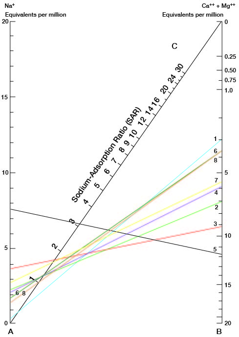
Figure 14--Classification of irrigation waters from representative wells in the Grant-Stanton area. (See Table 15 for well numbers.)
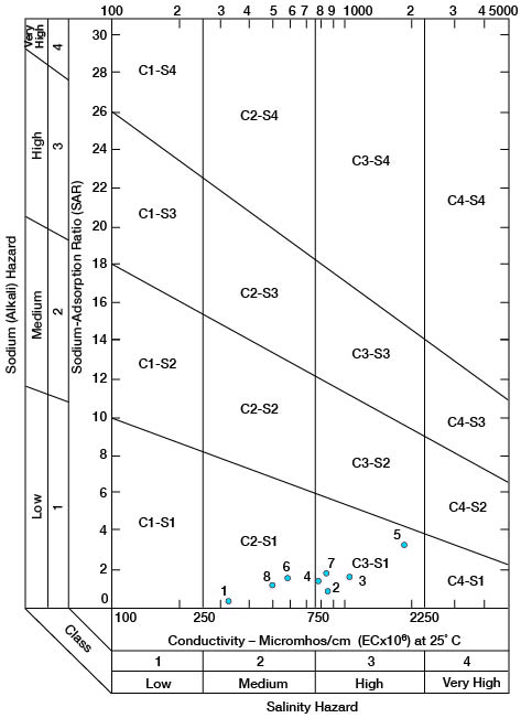
Table 15--Index numbers of samples shown in Figures 13 and 14 and sodium adsorption ratio (SAR).
| Well number | Number used in Figures 13 and 14 |
Geologic Source1 | SAR |
|---|---|---|---|
| 27-35-24ac | 1 | Npl, No | 0.3 |
| 27-39-13ac | 2 | Kd, Kc | 1.3 |
| 28-38- 4cc | 3 | Npl, No | 1.7 |
| 29-35-15ab | 4 | Npl | 1.3 |
| 29-36-23ddd | 5 | Npl | 3.1 |
| 29-36-30bc | 6 | Npl, No | 1.3 |
| 29-42-Ildc | 7 | Kd, Kc, TRd | 1.6 |
| 30-37-36bc | 8 | Npl | 1.0 |
| 1. Npl, Pleistocene; No, Ogallala Formation; Kd, Dakota Formation; Kc, Cheyenne Sandstone; TRd, Dockum Group. |
|||
Low-sodium water (S1) (Fig. 14) can be used for irrigation on almost all soils with little danger of developing harmful levels of exchangeable sodium. Medium-sodium water (S2) can be used safely on coarse-textured or organic soils having good permeability, but it will present appreciable sodium hazard in certain fine-textured soils, especially those not leached thoroughly. High-sodium water (S3) may produce harmful levels of exchangeable sodium in most soils and will require special soil management, such as good drainage, thorough leaching, and addition of organic matter. Very high sodium water (S4) is generally unsatisfactory for irrigation unless special action is taken, such as addition of gypsum to the soil.
Low-salinity water (C1) can be used for irrigation of most crops on most soils with little likelihood that soil salinity will develop. Medium-salinity water (C2) can be used if a moderate amount of leaching occurs. Crops of moderate salt tolerance, such as potatoes, corn, wheat, oats, and alfalfa can be irrigated with C2 water without special practices. High-salinity water (C3) cannot be used on soils with restricted drainage. Very high salinity water (C4) can be used only on certain crops and then only if special practices are followed.
The irrigation water being used in the area is a low-sodium water, (Fig. 14) but it is medium to high in salinity.
Phreatophytes
A plant that habitually obtains its water supply from the zone of saturation, either directly or through the capillary fringe, is termed a phreatophyte (Meinzer, 1923, p. 55). The Subcommittee on Phreatophytes (1958, p. 5,) states, "A phreatophyte in most cases is a mesophyte which grows in arid or semi-arid climates and which gets its water supply from ground water." The most abundant phreatophytes in this area are salt cedar (five-stamen tamarisk), willows, and cottonwoods. In some parts of the west these plants grow along valleys and flood plains and use considerable water. These plants, the tamarisk in particular, are of little or no economic value and grow thick enough in some areas to choke the stream channels, causing flooding. The tamarisk is difficult to control once growth has started, and care should be taken not to spread this plant deliberately.
Tamarisks, willows, and cottonwoods grow in abundance along the Arkansas River as far east as Dodge City, Kansas. It is not known how far they extend down the Cimarron River, but a few grow near Wagon Bed Springs south of Ulysses. Figure 15 shows the areas where tamarisks are growing in the Grant-Stanton area.
Figure 15--Map showing occurrence of phreatophytes in the Grant-Stanton area. (Areas of phreatophytes shown in black and indicated by arrows.) A larger version of this figure is available.

Prev Page--Formations || Next Page--Conclusions
Kansas Geological Survey, Geology
Placed on web July 23, 2007; originally published December 1964.
Comments to webadmin@kgs.ku.edu
The URL for this page is http://www.kgs.ku.edu/General/Geology/Stanton/06_hydro.html