Previous--Midcontinent Rift System || Next--Amplitude Variation with Offset
1Department of Geology and Geophysics, University of Missouri-Rolla, 2Consultant, Wichita, and 3Kansas Geological Survey
This article available as an Acrobat PDF file (6 Mb).
Geological bodies such as reefs, horst blocks, channel sandstones, faults, salt diapirs, deltaic complexes, etc., typically generate recognizable seismic signatures (or distinguishing seismo-geological features). The seismic signature of a geological body (a reef, for example) is composed of any and all features on the seismic data that can be confidently attributed to the presence of the reef.
Seismic signatures have two basic components: time-structure variations and character variations. The time-structure variation component is created by structural relief in the subsurface and velocity-generated, time-structural relief (pull-up/push-down effects). The character variation component consists of lateral changes in the amplitude and/or phase of specific events and lateral variations in the seismic image of specified units (typically corresponding to stratigraphic groups). The seismic image of a specified layer is the pattern of the sequence of events from the top to the base of that layer, inclusive.
Forward seismic modeling is the process through which a geologic section (subsurface depth! density/acoustic-velocity model) is transformed into a synthetic seismogram, thereby enabling the relationships between the subsurface and the corresponding synthetic seismogram to be deduced. Such modeling can elucidate the potential utility of the seismic technique prior to the acquisition of field seismic data and facilitate the interpretation of acquired data. Seismic modeling is typically done both before and after the acquisition of seismic field data. It aids the planning of an acquisition program and it is essential in interpretation, making correlation of the observed reflections with geologic interfaces possible, and verifying the seismic responses of deduced anomalies.
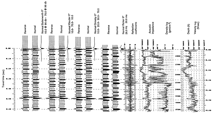
Forward seismic modeling is the process through which a geologic section (subsurface model of one, two, or three dimensions) is transformed into a synthetic seismogram (synthetic seismic record). Depth and acoustic impedance (product of velocity and density) variations within the geologic section are converted to transit time and reflection amplitude, respectively (fig. 1). The relationship between the geologic section and the corresponding synthetic seismogram can then be deduced. Such modeling can elucidate the potential utility of the seismic technique prior to the acquisition of field seismic data and facilitate the interpretation of acquired data. Seismic modeling is typically done both before and after the acquisition of seismic field data. It aids the planning of an acquisition program, and it is essential in interpretation, making correlation of the observed reflections and geologic interfaces possible, and verifying the seismic responses of deduced anomalies.
Figure 1--Velocity log, density log, acoustic impedance curve (product of seismic velocity and density), reflection coefficient curve (acoustic impedance contrast) and suite of synthetic seismograms for the sec. 2, T. 30 S., R. 24 W. well. Each synthetic seismogram is generated by convolving the reflection coefficient curve with different type of zero-phase wavelet (ie. Ricker, Orsmby, Klauder, Butterworth). Such one-dimensional synthetic seismograms are generally used to correlate field seismic data to the subsurface geology. Note that in all of the figures, positive acoustic impedance contrasts (higher values with increasing depth) generate peaks (deflections to the right); the "arrival time"of a zero-phase wavelet is measured at the apex of the respective trough or peak. Transit time is two-way travel time.
Seismic surveys are usually designed with one or more geologic objectives in mind. Modeling is typically done prior to the acquisition of seismic data to ensure that the geologic objectives are potentially seismically visible and to ensure that appropriate field acquisition parameters are used.
Modeling prior to acquisition gives a good indication whether we will be able to resolve the geologic objective, assuming we manage to obtain good-quality field data. It can verify or refute whether geologic objectives can be seen within the limits of the field techniques that will be used. We will probably be able to identify our geologic objective on real seismic data if its seismic image can be resolved on synthetic seismograms.
The seismic interpreter conceptually transforms seismic sections into geological sections. Reefs, horst blocks, channel sandstones, faults, salt diapirs, deltaic complexes, etc., are typical geologic targets, the seismic image of which the experienced explorer intuitively inverts (transforms seismic time sections into depth sections). The interpreted seismic data must result in geologic sections that are consistent with well log data and/or other geologic control.
Typically, synthetic seismic data are generated for all or part of a subsurface geologic section (as initially envisioned). The synthetic seismogram is compared to the real seismic data. When significant discrepancies are observed, the geologic section is modified (within the constraints imposed by other independent control) and a new synthetic seismogram is generated. This process is iteratively repeated, until the interpreter is satisfied with the correlation between the synthetic seismogram and the real seismic data, and is confident of the final interpretation.,
Geological bodies or exploration targets such as reefs, horst blocks, channel sandstones, faults, salt diapirs, deltaic complexes, etc., typically generate recognizable seismic signatures (or distinguishing seismo-geological features). The seismic signature of a geological body, a reef, for example, is composed of any and all features on the seismic data which can be confidently attributed to the presence of the reef.
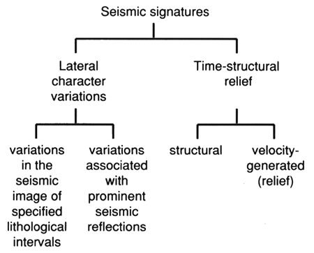
Seismic signatures have two basic components: time-structure variations and character variations (fig. 2).
Figure 2--Components of the seismic signature of a geological body can be categorized as "lateral character variations" or "time-structural relief."
The time-structural component of the seismic signature of a geological feature is due both to subsurface relief (fig. 3) and to velocity-generated, time-structural relief (figs. 4 and 5).
Figure 3--Structural relief in the subsurface is manifested as time-structural relief on seismic data. in the upper illustration (geologic section), horizon 2/1 is displayed on a depth section; in the lower diagram (synthetic seismogram), horizon 2/1 is displayed on the corresponding time-section. The apex of the zero-phase Ricker wavelet peaks represents the arrival time of the event on the synthetic seismogram. The amplitude and polarity of the reflection is a function of the acoustic impedance contrast (product of velocity and density) between layers 2 and 1. In the process of "inversion," subsurface velocity functions and reflection amplitudes are used to convert seismic data into depth sections.
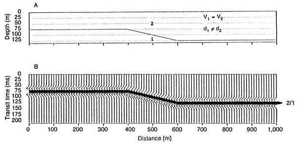
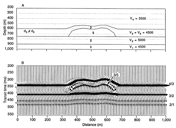
Figure 4--Lateral variations in the acoustic velocity of the subsurface generate timestructural relief on seismic data. in the upper iuustration (geologic section), horizons 2/1 and 3/2 are displayed on a depth section; in the lower diagram (synthetic seismogram), these horizons are displayed on the corresponding time-section. Note that the time-structural relief observed along the events (reflections) 3/2 and 2/1 are due to lateral velocity variations within layer 3.
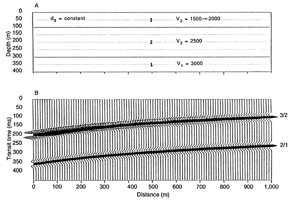
Figure 5--Time-structural relief along event 4/3 is due to structural relief. Time-structural relief along event 2/1 is attributable to lateral variations in the thicknesses of the overlying layers.
Subsurface relief may be the result of such features as primary depositional patterns, post-depositional deformation (faulting, folding, uplift, diapirism), erosion, salt dissolution, differential compaction, etc.
Velocity-generated, time-structural relief is primarily due to lateral facies variations and lateral variation in the thickness of a sediment of relatively uniform velocity. For example, the thickness of a channel sandstone can vary from 0 m to 30 m (0 ft to 100 ft) over a distance of less than a few hundred meters. Depending upon the velocity contrast between the channel sandstone and the encasing sediment, and associated structural relief, the pre-channel horizons may be "pulled-up" or "pushed down" beneath the channel facies.
When seismic modeling is done prior to data acquisition, the interpreter is attempting to determine' whether the time-structural relief component of the seismic signature of the geological objective will be visible on field seismic data. When modeling is done after the acquisition of the data, the interpreter is trying to determine the nature of the geological feature that generated the observed pattern of time-structural relief.
A word of caution: a component of time-structural relief on field seismic data can result from inappropriate statics corrections, too little care in processing, or over-zealous processing (figs. 6 and 7).
Figure 6--Apparent time-structural relief can be caused by the application of inaccurate elevation or weathering corrections. Elevation corrections account for lateral changes in the surface elevation of shot and receiver locations; weathering corrections account for the lateral velocity variations which are characteristic of the shallow subsurface in many places.
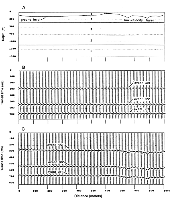
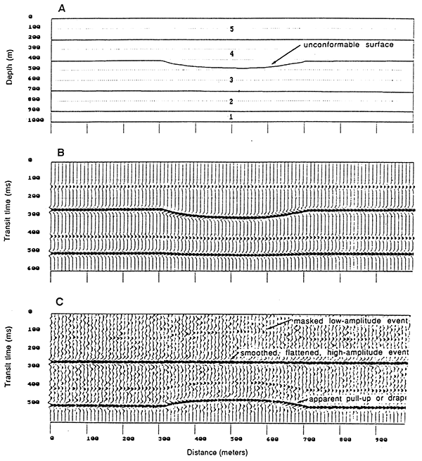
Figure 7--Apparent time-structural relief can be an artifact of processing. In the middle diagram the geologic section has been properly transformed into a synthetic seismogram. The lower diagram is intended to illustrate the situation where a processor has used the high-amplitude reflection from the unconformable surface as a datum (20% noise has been superposed on the synthetic seismogram). As evidenced by the figures, such injudicious processing techniques can lead to erroneous interpretations.
Character variations can be classified as lateral changes in amplitude and/or phase along a specific seismic event, or as lateral changes in the seismic image of a specified unit. Amplitude and/or phase variations typically occur as a result of constructive and destructive interference (figs. 8 and 9), lateral variation in acoustic impedance contrast (fig. 10), focusing and defocusing (fig. 11), diffractions (fig. 12) and differential attenuation. Lateral variations in the seismic image of a specified unit typically result from facies variation within that zone (e.g., reef to off-reef transition; fig. 12). Character variations that are independent of the body of interest are not considered to be components of the seismic signature of that body. These include interference from noise and some multiples (figs. 12 and 13).
Figure 8--Amplitude variations can occur as a result of constructive interference or "tuning." On the synthetic seismogram, the reflections from horizons 3/2 and 2/1 are seen to visually merge as layer 2 pinches out from left to right. At trace 100 (one wavelength separation on geologic section), these events are distinct; from trace 99 to 50 (approximately one-half wavelength separation), the troughs which trail and precede the dominant peaks of the zero-phase Ricker wavelets increasingly constructively interfere. Thereafter, until the vicinity of trace 25, these same troughs destructively interfere with the dominant peaks to an increasing degree; the width of the wavelets appears to decrease and the apex of the upper and lower peaks (interpreted as the "arrival" time of the events) appears to be deflected upwards and downwards, respectively. Between traces 25 and 1, the dominant peaks begin to visually merge from a wide "doublet" into a single high-amplitude peak.
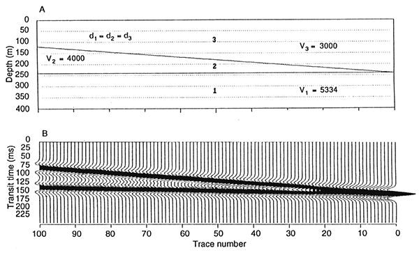
Figure 9--Amplitude variations can occur as a result of destructive interference. On the synthetic seismogram, the equal amplitude and opposite polarity events 3/2 and 2/1 visually merge from left to right. At trace 1, these reflections superpose and cancel, yielding a null trace.
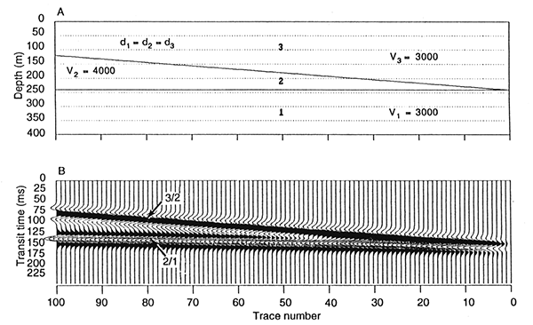
Figure 10--Amplitude variations along a specific reflection can occur as a result of lateral changes in acoustic impedance contrast. In the model, the amplitudes and polarities of events 2/3 and 1/2 change from left to right as a result of a change in the seismic velocity of layer 2.
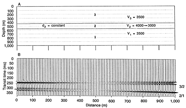
Figure 11A---Geologic section and corresponding vertical incidence synthetic seismogram (analogous to ideally migrated seismic data). Dipping surfaces are accurately located in time and space on this synthetic seismogram.
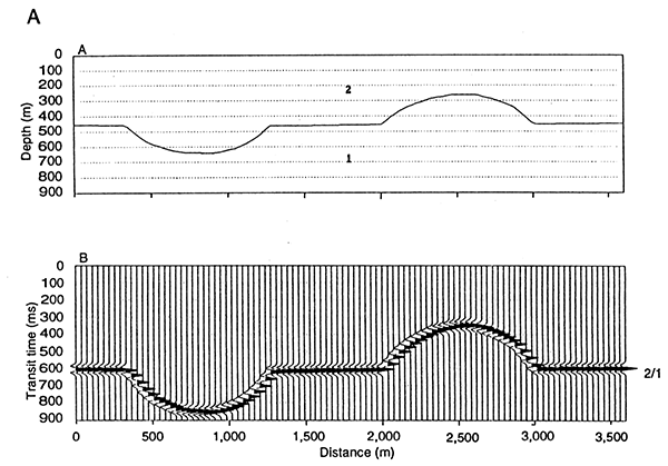
Figure 11B---Geologic section and corresponding diffraction synthetic seismogram (analogous to non-migrated seismic data). Dipping surfaces are shifted in time and space; anticlinal structures are broadened and synclinal features are collapsed. Diffractions originating from discontinuities within the geologic section are superposed on the reflections. Note in this model the focal point of the syncline (as illustrated by the raypaths) is above ground level.
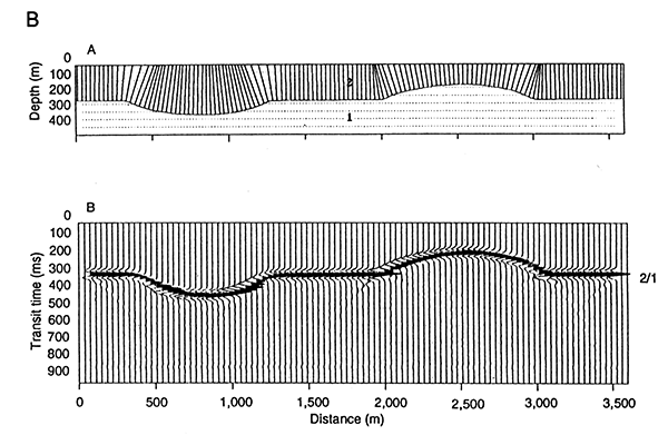
Figure 11C--In this model the focal point of the syncline is near ground level at receiver 75. As a result of focusing, the amplitude of the reflection on trace 75 is magnified. Diffractions originating from discontinuities within the geologic section are superposed on the reflections.
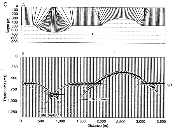
Figure 11D--In this model the focal point of the syncline is situated below ground level. in this situation, the superposed reflections from the syncline and the diffractions emanating from the associated edge discontinuities are manifested as a classic "bow-tie."
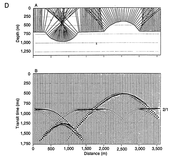
Figure 12A-E---Geologic model and corresponding suite of synthetic seismograms. In B, a diffraction synthetic seismogram is shown. The diffractions originate from discontinuities associated with the surface of the reef and are considered to be part of the seismic image of the reef. In C, a vertical incidence synthetic seismogram is depicted. Note how definitively the seismic image of the reef can be differentiated from that of the laterally adjacent strata. In D and E, random noise has been superimposed on the vertical incidence synthetic seismogram. Noise (everything other than desired signal) is not considered to be part of the seismic signature. Frequency filtering, stacking, geophone arrays, and processing techniques are used to increase the signal-to-noise ratio. These two-dimensional synthetic seismograms are often generated in order to elucidate the utility of seismic technique with respect to exploration for an envisioned geologic target.
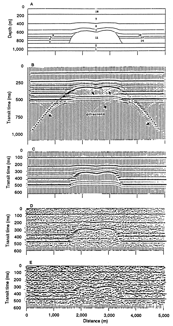
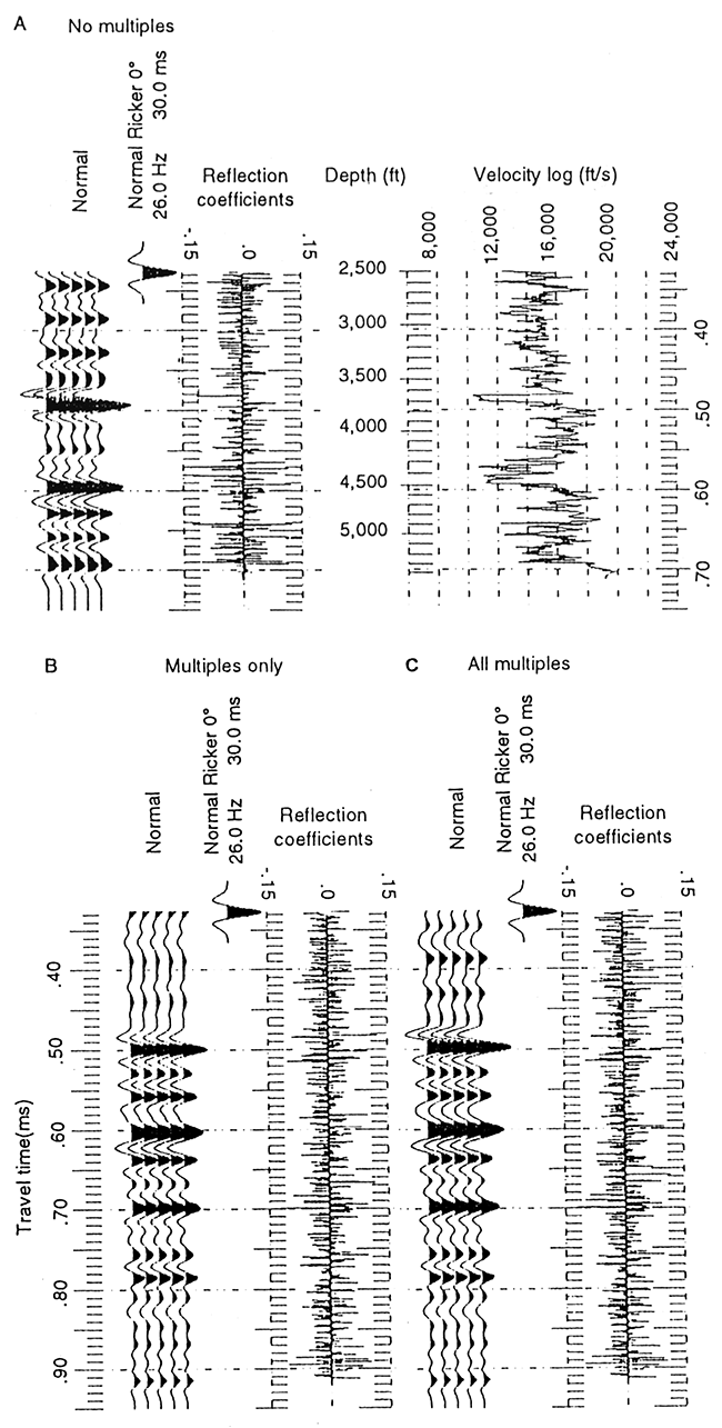
Figure 13A-C--One dimensional velocity/depth log (sec. 2, T. 30 S., R. 24 W. well) and corresponding suite of vertical incidence synthetic seismograms: A--primary reflections only, B--primary reflections and all multiples, and C--multiples only. Multiples can mask the seismic signature of a geologic target; they are generally considered to be noise. CDP stacking and processing techniques are used to reduce the relative amplitudes of multiple events.
When seismic modeling prior to data acquisition, the interpreter is attempting to determine whether the character variation component of the seismic signature of the geological objective will be seismically visible. When modeling after data acquisition, the interpreter is generally attempting to deduce the geological origin of an observed seismic anomaly.
Seismic data are usually acquired to delineate a preconceived geological objective. Generally, the survey area has been selected on the basis of geological studies and is considered to be a favorable area with respect to the envisioned target. Pre-acquisition modeling consists of transforming the envisioned subsurface geologic section (subsurface model with units of depth, acoustic velocity, and density) into a synthetic seismic section (composed of space (0-, 1-, or 2-dimensions), time, and units of reflection amplitude). Typically, if the seismic signature of a geological target is not manifested on appropriately modeled synthetic seismograms, it will not be seen on field seismic data. Whether modeled features are interpretable on resultant seismic data depends largely upon the accuracy of the geologic section and the quality of the real seismic data (function of noise, multiple interference, acquisition parameters, quality of processing, etc.).
There are two types of pre-acquisition geologic sections-stratigraphic and structural. Both are designed on the basis of well control in the immediate vicinity of the study area, regional trends, the morphology, and acoustic impedance characteristics of features similar to the envisioned target. The stratigraphic and structural sections generally differ with respect to detail and ultimate purpose. Stratigraphic sections are designed to provide information with respect to the character variation component of the seismic signature of the envisioned anomaly. In contrast, structural sections are designed to illustrate the time-structural relief component. Typically, the stratigraphic section is restricted to that portion of the subsurface in the immediate vicinity of the envisioned geological anomaly, whereas the structural section usually extends from the surface to a depth below the features of interest.
Stratigraphic synthetic seismograms are generated in an effort to determine whether the character variation component of the seismic signature of the geological target will be seismically visible (figs. 1 and 13). Structural synthetic seismograms are usually generated in order to determine whether the time-structural component of the seismic signature of the geologic target will be visible (fig. 12).
In the case of the stratigraphic synthetic seismograms, modeled amplitude and phase variations along specific events and changes in the seismic image of layers are closely analyzed. In the case of the structural synthetic seismograms, the modeled seismic response to subsurface structure and velocity-generated time-structural relief are analyzed. Based on these analyses, the interpreter decides whether the seismic signatures of the geological objective should be visible, assuming appropriate field acquisition parameters are employed, sufficiently good quality field data is obtained, and the data are properly processed.
Whether seismic signatures can be distinguished on the field data is a function of both the quality of the field data and signal/noise ratio of seismic data. Subtle or weak anomalies might only be seen on the final processed section. However, likely key marker horizons are noted on the synthetic seismograms and examined on common shot records (field seismograms) as a check of data quality.
Pre-acquisition modeling can be thought of as a precautionary measure-the seismic interpreter is attempting to safeguard against acquiring data in search of a target that is not likely to be visible on real seismic data and against using inappropriate field acquisition parameters.
Seismic data are usually acquired to delineate a preconceived geological objective. Generally, geologic sections (subsurface models) of such envisioned targets have been generated prior to data acquisition in order to ensure (within reason) that the seismic signature of the target will be visible on reasonable quality seismic data and as an aid to the design of field-acquisition parameters.
During post-acquisition modeling, the seismic interpreter, intuitively or otherwise, inverts the interpreted seismic data and develops a geological section using all available data as constraints. Such data would include acoustic and density log data, drilling and lithology data, stacking velocities, and check shot velocities. Experience and intuition will assist in refining modeled geologic sections.
A synthetic seismogram is generated by the interpreter for all or part of the geologic section and compared to the processed seismic data. When discrepancies are observed, the geologic section is modified and a new synthetic seismogram is generated. This process is iteratively repeated, until the interpreter is satisfied with the correlation between the synthetic seismogram and the real seismic data. Care must be taken to ensure that the final output is consistent with known geological constraints.
There are two complementary types of post-acquisition models-stratigraphic and structural. Both are designed on the basis of the inverted seismic data (intuitive or otherwise) and are constrained by available knowledge, including well log control, check shot velocities, regional trends and morphology, and acoustic impedance characteristics of related geological features. Stratigraphic models are generated to clarify the geological origin of the character variation component of an observed seismic anomaly. Structural models are generated to determine the origin of the time-structural component of an observed anomaly.
The stratigraphic synthetic seismogram enables amplitude and phase variation along specific events and variations in the seismic images of specific layers to be closely analyzed. Accuracy can depend on knowledge of the wavelet of the seismic energy pulse, that is, the response to a hypothetical isolated reflector. Using the structural synthetic seismograms, the interpreter attempts to deduce structural relief in the subsurface and to determine the velocity variations which produced the observed pattern of velocity-generated time-structural relief. This later seismogram depends on a stable wavelet on the real seismic data but is not dependent on identification of the wavelet form.
Post-acquisition modeling can similarly be thought of as a precautionary measure. The interpreter is attempting to ensure that anomalous features on the seismic data, in all probability, originate from geological features worthy, of further evaluation (i.e., the acquisition of additional seismic control, drilling, etc.). The interpreter is attempting to avoid the gross error of an unrealistic interpretation.
Through forward seismic modeling, the interpreter can elucidate the potential utility of the seismic technique prior to the acquisition of field seismic data and thereafter facilitate the interpretation of acquired seismic data. Seismic modeling is typically done both before and after the acquisition of seismic field data. It aids the planning of an acquisition program, and it is essential in interpretation, making correlation of the observed reflections and geologic interfaces possible and verifying the seismic responses of deduced anomalies.
There are two basic types of forward models-stratigraphic and structural. Both are designed on the basis of well control in the immediate vicinity of the study area, regional trends, the morphology, and acoustic impedance characteristics of features similar to the envisioned target. The stratigraphic and structural synthetic seismograms generally differ with respect to detail and ultimate purpose. Stratigraphic synthetic seismograms are designed to provide information with respect to the character variation component of the seismic signature of the envisioned anomaly. In contrast, structural synthetic seismograms are designed to illustrate the time-structural relief component. Typically, the stratigraphic seismogram is restricted to that portion of the subsurface in the immediate vicinity of the envisioned geological anomaly, whereas the structural seismogram usually extends from the surface to a depth below the features of interest.
Previous--Midcontinent Rift System || Next--Amplitude Variation with Offset
Kansas Geological Survey
Comments to webadmin@kgs.ku.edu
Web version placed online Aug. 19, 2015. Original publication date 1995.
URL=http://www.kgs.ku.edu/Publications/Bulletins/237/Anderson1/index.html