Previous--Climate Change and Sustainable Water Yield || Next--Glossary
This article available as an Acrobat PDF file (148 kb).
"Doubt is not a pleasant state but certainty is a ridiculous one."
--Voltaire
There are few things in life that we are certain about (notably death and taxes), and water is not one of them. Of course, there will always be water: some of it, somewhere, for some time. However, for planning purposes we need to know how much water will be available, where, and when. Furthermore, we need to know it with a high degree of confidence in order to have reliable water supplies. There are two ways to know these things: either we measure or we estimate. But we do not always get to choose; some variables we can measure (e.g., water levels) and some we can only estimate (e.g., rock permeability). In both cases there can be significant uncertainty as to the actual values at a given time and location.
Uncertainty can be of two types: natural variability or lack of knowledge. Most people are familiar with uncertainty due to natural variability, as they evaluate weather forecasts on a daily basis. River stages are another example: we have years of daily records, but still cannot predict future water levels much in advance. However, rainfall, temperatures, and river stages are accessible to measurement; when we measure them, we register their natural variability. On the other hand, uncertainty due to lack of knowledge relates to things that we cannot measure but still affect the prediction to be made. This latter category is very pervasive in subsurface hydrologic systems, because we can seldom measure the variable that we need to predict. Examples include water yield and aquifer permeability.
Regardless of their origin, we deal with all uncertainties in a similar way. We only have two choices: ignore it or recognize it. The price of ignoring it can be too high in water-resources planning: we will fail to get the needed quantity of water. A better choice is to explicitly recognize all sources of uncertainty and evaluate their impact on the variables that we need to estimate (e.g., water yield). Because uncertainty and risk are companions, evaluating uncertainty allows the assessment of risks and management of its consequences.
Water-resources planners face an irreducible dilemma. They realize that our knowledge of the hydrologic system is fraught with uncertainties, but decisions still need to be made. The key question is: Will those uncertainties affect the decisions to be made? The only way to know is to incorporate uncertainty into the analysis in a quantitative fashion, by means of probabilities. This alternative is always superior to neglecting uncertainty to avoid dealing with it. By doing this, decision-makers can set policies that meet acceptable levels of risk. In this chapter, I advocate such an approach and show how this can be done using available information.
A simple example will serve to illustrate some basic ideas about uncertainty. Consider the daily discharges in the Kansas River near Lecompton. Sixty years of daily records, from 1937 to 1996, are summarized in fig. 9.1. Figure 9.1A shows the histogram of relative frequency; fig. 9.1B shows the cumulative relative frequencies (the maximum value of 1 corresponds to certainty). The relative frequency is the number of times a given value occurs, divided by the total number of observations. Both plots in fig. 9.1 provide a wealth of information: we observe not only the range of possible values (from 185 cfs to 398,000 cfs [5-11,270 m3/s]), but also the likelihood of observing values in a given interval. We can use the sample data to make inferences about particular events. However, to do that we first need to assign a likelihood to each event: this measure is called probability. In view of the sample data it seems reasonable to make the relative frequencies equal to the corresponding probabilities (this is true in the limit of large sample size). In what follows, we will use the term probability instead of frequency.
We wish to estimate the probability of a flood on any given day. To do this we need to group the information in fig. 9.1A into two exclusive events: smaller or larger than a given threshold value. This is done automatically in fig. 9.1B, which measures the probability of having discharges less than a given value. For example, we can read in fig. 9.1B a probability of 80% of having discharges smaller than 10,000 cfs. Because probabilities of complementary events add up to one, we calculate a probability of 20% of having a flood with discharges larger than 10,000 cfs.
Figure 9.1--Variability of daily discharges in the Kansas River at Lecompton. (A) Probability-density function (pdf). (B) Cumulative-distribution function (CDF).
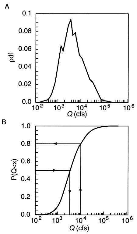
This example shows all the basics of dealing with uncertainty. Information can be grouped to display the relative likelihood of events of interest, including mutually exclusive events (e.g., discharges larger or smaller than a given value). Probabilities can be read directly from the cumulative distribution function (CDF) depicted in fig. 9.18. The CDF is obtained by adding up the values of the probability density function (pdf) depicted in fig. 9.1A. Risk is the probability of an undesirable event. We can either select the event and calculate the risk, as done above, or set the maximum acceptable risk level and determine the corresponding event. For example, in fig. 9.1B we read that a flood risk of 50% corresponds to a discharge of 3,300 cfs.
Water-yield estimates are the result of a hydrologic-balance calculation, based on the initial stock of water, the additions (e.g., precipitation), and subtractions (e.g., evaporation). Since these quantities vary over time, so does the water-yield estimate. This presents a potential problem for defining unique yield values to guide policy making. One possibility is to perform the balance calculations under long-term average conditions (which might materialize or not). This might be appropriate for groundwater systems with long response times, but not for systems that are relatively fast to respond to changes in major fluxes. For those systems, a better choice might be to evaluate yield under conditions of relative drought, when additions are much less than those during average conditions; this is perhaps the simplest way to hedge against the risk of running out of water.
Estimates of ground-water yield are always uncertain because-unlike river stages-they are not directly measurable. They are estimated using a model of the hydrologic system, in terms of other variables that are estimates themselves (by contrast, the yield from a surface-water reservoir has significantly less uncertainty). Here we use the term yield estimates to emphasize the fact that they are inherently uncertain.
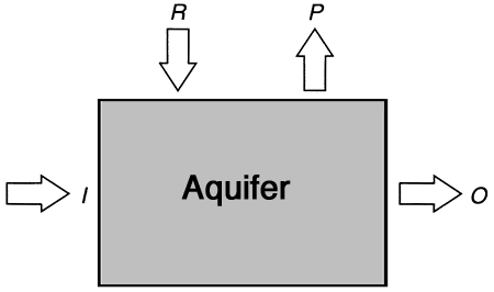
We will illustrate yield uncertainty by way of an example. Consider an unconfined aquifer subject to recharge from precipitation and otherwise not connected to surface-water bodies; an underlying aquitard prevents recharge from below. We wish to evaluate the feasibility of pumping water from this aquifer for irrigation, on a long-term equilibrium basis. This system can be described at different levels of detail; here we choose the simplest conceptualization using the lumped parameters shown in fig. 9.2. The corresponding steady-state mass-balance equation is
I + R - P = O (eq. 9.1)
where R is the recharge, P is pumping, I is the regional-flow input, and O the regional-flow output. Pumping is a decision variable that can take one of three possible values, P = {1; 2; 3}. Other available information allows us to estimate values of I and R as follows (all numerical figures in this example have the same arbitrary units):
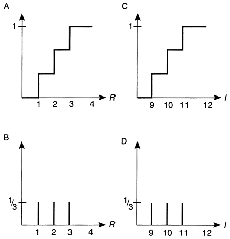
I = {9; 10; 11} mean [I] = 1
R = {1; 2; 3} mean [R] = 2
Figure 9.2--Box diagram depicting fluxes in and out of an aquifer: freshwater recharge (R), pumping (P), regional ground-water flow input (I), and regional ground-water flow output (O).
These values portray uncertainty in a very simple fashion: each variable can take on three possible values, all equally likely (each one has a probability of occurrence equal to 1/3). Because in reality both I and R are continuous variables, the three-point discrete representation can only approximate their true variability. However, the mathematics are much simpler, and we can still illustrate the same points. Figure 9.3 shows the relative frequency plots for I and R. There is a direct equivalence with the plots in fig. 9.1, but by custom the discrete functions have different names: the relative frequency plot is the probability mass function (pmf), and the cumulative one is the cumulative mass function (CMF). Otherwise we use them in much the same way as their continuous counterparts. The only difference is that the CMF has sudden jumps at points where the pmf is nonzero (fig. 9.3 shows vertical bars of height equal to 1/3 that describe the pmf of both I and R).
Figure 9.3--Uncertainty in the estimates of freshwater recharge R and regional ground-water flow input I, as measured with three-point probability mass functions (pmf) and cumulative mass functions (CMF). (A) CMF of recharge R. (B) pmf of recharge R. (C) CMF of groundwater-flow input I. (D) pmf of ground-water-flow input I.
We assume a realistic constraint on the regional flow output O: due to an agreement with the authorities of the down-gradient groundwater management district, O cannot be arbitrarily lowered to satisfy pumping needs. The agreement recognizes that uncertainty is a fact of life, and establishes a risk-based constraint: O has to equal or exceed nine units with a probability of 80% or better (if we assume that uncertainty is due to interannual variability, this constraint is equivalent to accepting that O can be less than nine units in one out of every five years, on average). Here risk is the probability of failing to meet the standard that O equals or exceeds nine units. Alternative standards could be expressed in terms of other variables, such as maximum water-level declines, maximum concentration of dissolved solids at the pump, etc. The novelty of this approach is that a (small) risk of noncompliance is accepted to build some flexibility into management policies. Knowing that the complement of risk is reliability, and that both quantities add up to unity, we can see that the above policy has a reliability of 80% and a risk of 20%.
Armed with this information, we can evaluate the behavior of the system with and without pumping. That is, using the above balance equation we calculate values of the output O, corresponding to each value of pumping P. Under predevelopment conditions (P = 0), I + R = O. Because I and R can each take on three different values, O can take on the following nine values: {10; 11; 12; 11; 12; 13; 12; 13; 14}. Each of the nine values is equally likely (each has a probability equal to 1/9), but some of them occur more than once. This can be easily accounted for by counting repeated occurrences and adding their original probabilities as shown in table 9.1; the resulting values of O and their probabilities are summarized in the following table and displayed in fig. 9.4B.
Table 9.1--Repeated occurrences of values of calculated output and their original probabilities.
| x | Prob[O = x] | Prob[O < x] |
|---|---|---|
| 10 | 1/9 | 0 |
| 11 | 2/9 | 1/9 |
| 12 | 3/9 | 3/9 |
| 13 | 2/9 | 6/9 |
| 14 | 1/9 | 8/9 |
Figure 9.4--Uncertainty in the estimates of regional groundwater flow output O in the absence of pumping, as predicted with a steady-state mass balance model. (A) Probability-mass function (pmf). (B) Cumulative-mass function (CMF).
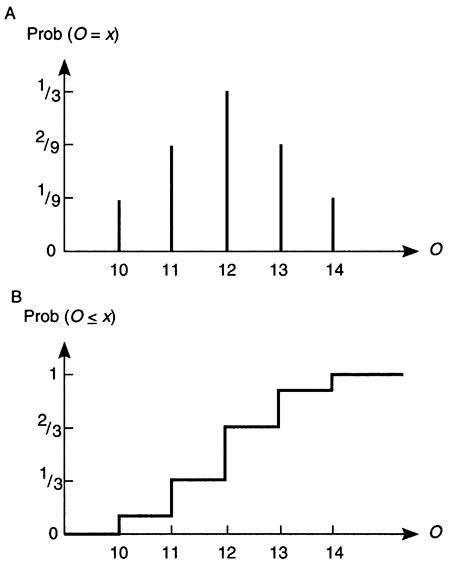
The corresponding cumulative probabilities, Prob[O < x], are obtained by adding up the individual values smaller than a given threshold, as shown in the last column of table 9.1 and plotted in fig. 9.4A. We can use this figure to evaluate the probability of compliance with the minimumflow requirement: the risk of having O less than nine units has to be smaller than 20%. Examination of fig. 9.4A reveals that the probability Prob( 0 < 9] is zero, because all values are larger than nine units. Then, in the absence of pumping, this constraint is easily met.
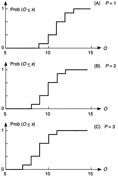
To analyze the impact of pumping, we simply repeat the calculation of O for different values of P. The results are displayed in fig. 9.5 and shown in table 9.2. From table 9.2 we can read the probability of compliance with the minimum flow requirement, for each value of P. We observe that when P = 3 the requirement is not met, since Prob[O < 9] = 3/9 = 33%. However, P = 2 is acceptable, because Prob[O < 9] = 1/9 = 11%.
Now examine the alternative of neglecting uncertainty. We change the risk-based constraint to an equivalent deterministic one: the output 0 can have a minimum value of 10 units. We adopt the mean values for I and R (J = 10; R = 2), and find out that a pumping level of P = 2 units is acceptable. By coincidence this value is the same as the one determined with full knowledge of uncertainty. However, there is a large chance (1/3) that O will be less than 10 units, as shown in table 9.2 and in fig. 9.5. In other words, we are taking a risk of 33% of not meeting the minimum-flow requirement, but we do not know it. In general we can expect such apparently risk-neutral policies to carry an even larger risk (called risk-neutral because uncertainty and risk are neglected altogether). We can easily see that this is true even in the above example.
Table 9.2--Probability of compliance with minimum flow requirement for each value of pumping (P).
| P = 1 case: | x | Prob[O = x] | Prob[O < x] |
|---|---|---|---|
| 9 | 1/9 | 0 | |
| 10 | 2/9 | 1/9 | |
| 11 | 3/9 | 3/9 | |
| 12 | 2/9 | 6/9 | |
| 13 | 1/9 | 8/9 | |
| P = 2 case: | x | Prob[O = x] | Prob[O < x] |
| 8 | 1/9 | 0 | |
| 9 | 2/9 | 1/9 | |
| 10 | 3/9 | 3/9 | |
| 11 | 2/9 | 6/9 | |
| 12 | 1/9 | 8/9 | |
| P = 3 case: | x | Prob[O = x] | Prob[O < x] |
| 7 | 1/9 | 0 | |
| 8 | 2/9 | 1/9 | |
| 9 | 3/9 | 3/9 | |
| 10 | 2/9 | 6/9 | |
| 11 | 1/9 | 8/9 |
Figure 9.5--Uncertainty in the estimates of regional groundwater-flow output O for three different levels of pumping P, as predicted with a steady-state mass-balance model. Cumulative-mass functions are shown for (A) P = 1, (B) P = 2, (C) P = 3.
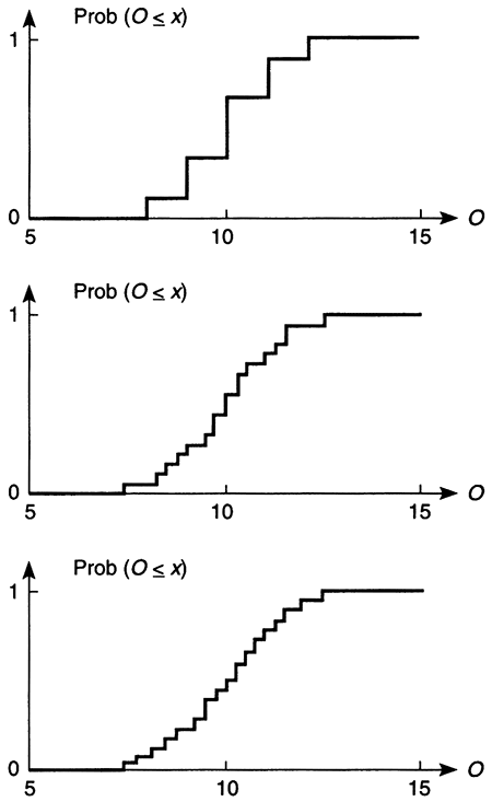
Imagine that we improve the resolution of our estimates by using more than three points to represent both I and R; the result will be a CMF with more steps than those in fig. 9.5. As we increase the number of points, the CMF approaches a smooth curve, while the mean value of O approaches 10 units; this process is schematically depicted in fig. 9.6. In a symmetric distribution, this means that there is a risk of about 50% of having actual values smaller than 10 units!
Figure 9.6--Distribution of regional ground-water-flow output O for pumping P = 2. Schematic illustration of the effect of refining the calculation by using more points to represent the variability of both recharge R and regional ground-water-flow input I.
Review the essence of the previous two examples. We recognized that each problem had a significant component of uncertainty and chose to incorporate it into the analysis. We tested a simple way to quantify uncertainty by means of three-point discrete distributions for each uncertain quantity. We learned how to graphically display information about uncertain quantities in terms of appropriate probability distributions (pdf and CDF for continuous, and pmf and CMF for discrete quantities). We also evaluated a risk-based constraint and made a decision based on it. In a nutshell, we learned a proactive approach to uncertainty management and decision-making under uncertainty.
The two examples illustrate that dealing with uncertain quantities is not a complicated process. However, it requires a sustained interest in exploring all possibilities, and a determination not to discard information too early in the process. By seeking and preserving the most information, we can present more alternatives to the decision makers, who can then make choices in terms of the risk level that they deem acceptable. This approach is superior to the alternative, where one makes a decision disregarding uncertainty and then hopes that the actual risk will turn out to be small.
On the other hand, there is a small price to pay to incorporate uncertainty in analyses and quantify the risk of alternative decisions. First, we may need to entertain more complex models of the hydrologic system in order to incorporate all possible sources of uncertainty. Second, we need to seek more information to define a range of values for each quantity (instead of a single estimate). However, this is not hard to do: all we need are realistic upper and lower bounds. With these bounds and a best estimate for each quantity, we can easily conduct a three-point uncertainty analysis, as demonstrated in the groundwater-yield example.
There is more to decision-making under uncertainty than the regulatory framework used in this example, where we assumed that an acceptable risk level had already been fixed. In most cases, decision-makers will evaluate the tradeoff between risks and consequences, often considering a suite of decision variables. There are many ways to combine disparate quantities in a single criterion, which can then be optimized to reduce the risk of an adverse event (cost-benefit analysis is a well-known example). An important advantage of using such a unified framework is that the impact of procuring additional information can be measured in terms of whether it can change the optimal decision (these are known as value-of-information analyses).
This points to the fact that uncertainties are not important per se, but only to the extent that they change the decisions to be made. This is especially important in water-resources management; we could be rather uncertain about some aspect of the hydrologic system, but if this uncertainty does not change the decision, it becomes irrelevant for management purposes. For this reason it is crucial to propagate uncertainties in the analysis all the way to the decision-making step. This also makes life easier because we do not need to decide a priori which uncertainties are of scientific interest and which of management relevance; this is decided automatically in the framework of decision-making under uncertainty.
In the ground-water-yield example, we used the simplest possible balance model to determine an acceptable water yield (pumping rate). This was useful to illustrate the main concepts, but hardly realistic as to the type and amount of information that would be needed in practice. Dealing with more information requires hydrologic models that incorporate more details of the natural system, and this means more sources of uncertainty. In this section we review some of those sources and their impact on ground-water-yield estimation.
A hydrologic model is always a simplified representation of the real system. Regardless of the scale of phenomena included in the model, details at smaller scale are not explicitly represented. If necessary they can be accounted for as additional uncertain variables. For example, spatial variability in aquifer properties can be represented in reasonable detail at the scale of a well field, but disregarded at the basin scale. Although average property values can be used at the basin scale, we can still preserve some information on its variability by treating it as an uncertain variable.
Consider a ground-water model. Once the scale and the spatial boundaries of the model are selected, we deal with four types of quantities: inputs, outputs, parameters, and decision variables. Decision variables, such as pumping rates, are controlled by the decision-makers and therefore carry no uncertainty. Outputs, such as water-table elevation, are the measures of system response predicted by the model; as we have seen, the model can predict uncertainty in outputs if desired. Then, it is only inputs and parameters that we need to assess as uncertain quantities. In the rest of this section we discuss model inputs and parameters as sources of uncertainty, and their impact on the uncertainty of model outputs, such as water yield.
Parameters of a ground-water model are related to the geology: thickness and spatial extent of aquifers and aquitards, lithology, porosity, permeability, etc. These quantities are spatially variable and only accessible to measurement at selected locations; at other locations we may obtain estimates by interpolation. Such estimates can then be treated either as perfectly known or as uncertain quantities in the model. Depending on the scale of the model, more than one spatially variable quantity may have to be considered. For example, uncertainty in hydraulic conductivity is relevant at the local scale (e.g., a well field); at the regional and basin scale other variables, such as formation thickness and horizontal continuity, compound their uncertainty to make the aquifer transmissivity an uncertain variable.
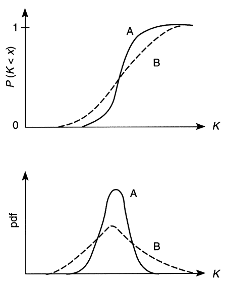
Figure 9.7 illustrates the natural variability in hydraulic conductivity in an aquifer, obtained from core samples (this distribution can also be interpreted as a measure of the uncertainty at unmeasured points in the same aquifer). The figure shows two distributions with the same mean value but different spread about the mean. Depending on whether the real distribution follows curve A or B, the ground-water system will behave very differently, and calculations that rely only on the mean value will miss significant information. Curve B has a larger spread than curve A, and therefore more extreme values on both ends of the spectrum displayed in fig. 9.7; the left tail of curve B corresponds to K values of smaller magnitude than the smallest values in curve A, while the right tail represents the reverse situation. The larger hydraulic-conductivity values at the right tail in curve B will correspond to larger velocity and shorter travel times than in curve A. This will affect yield estimates when subject to water-quality constraints. For example, if salinity transport from underlying aquifers is of concern, the critical travel time will be measured from a salt source to the point of interest, such as a well or a gaining stream.
Figure 9.7--Heterogeneity in hydraulic conductivity K in a single aquifer. Two distributions with the same mean but different standard deviation.
Inputs of a ground-water model are a diverse group of variables. They include water fluxes in and out of the model area, and water levels at reference locations such as lakes and streams. Water levels are regularly measured and carry little uncertainty, while fluxes are usually estimated and may carry significant uncertainty. Inflows to a ground-water model include incoming regional flow, recharge from underlying aquifers, and freshwater recharge from precipitation. Outflows include outgoing regional flow, discharge to streams, and pumping wells. These model inputs reflect the influence of external processes on the ground-water system, among them human activities and climate.
As discussed in Chapters 2 and 4, estimating groundwater yield is highly dependent on estimates of groundwater recharge and discharge change, which are subject to considerable uncertainty even under stable climatic conditions. Recharge estimates should reflect the natural variability in precipitation and temperature, with seasonal and multi-year cycles. Climate change would greatly increase the uncertainty in recharge estimates; this effect can be so dramatic as to overwhelm the uncertainty due to natural variability under a stable climate (see Chapter 8).
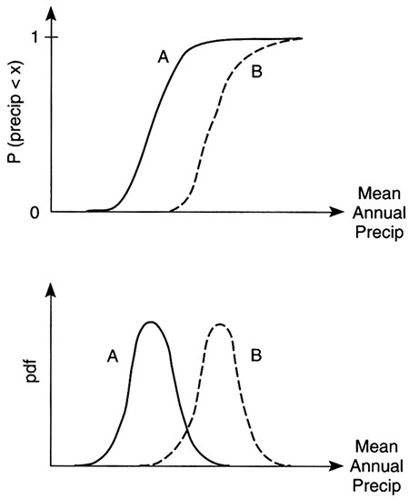
Estimating uncertainty in climate-related variables such as precipitation, temperature, and evapotranspiration presents unique difficulties. The primary reason is that we have to make inferences based on relatively short records (a hundred-year-long record is short in terms of climate processes). These records can capture at best some of the natural variability, but they provide no information about periods of qualitatively different climate. However, a number of such scenarios can be obtained from climate models and appropriately translated into ground-water models in terms of freshwater recharge. For example, we might want to examine the impact of an increase in precipitation. Figure 9.8 displays one possible scenario, where the whole distribution of mean annual precipitation is assumed to have shifted by a constant amount (curve A is the original distribution; curve B is the shifted one with a larger mean value). Under the scenario represented by curve B, wet years will have larger precipitation, while dry years will not be as dry as earlier (both in comparison to curve A). By conducting quantitative analyses like these, we can incorporate a realistic source of uncertainty that is not based on past data, but on analysis of possible futures.This is a type of knowledge uncertainty that we can only uncover through what-if analyses. The same applies to changes in land-use and agricultural practices.
Figure 9.8--Effect of climate change on the distribution of mean annual precipitation, assuming that all values are increased by the same constant amount.
Uncertainties in model inputs and parameters translate into uncertainty in those variables chosen as model outputs. Examples include water-level decline, groundwater discharge to streams, and salt content. Existing records for such variables provide a summary of system response, which can be useful to calibrate or constrain model parameters. However, the response is not immediate and there is always a lag between changes in inputs and the corresponding changes in outputs. Ground-water flow and transport processes reflect changes in inputs, according to their own characteristic time scales. Ground-water flow adjusts to changes in pumping and/or regional recharge within a time period that depends on the average aquifer properties at the appropriate scale. For example, a pumping well in the Dakota aquifer may take months or years to generate a steady-state-capture zone (see fig. 4.18). An example at the basin scale is the depletion time, which can be calculated with the linear-reservoir model (see fig. 2.8).
Water managers need to assess typical time scales such as these to characterize the transient response of the system before evaluating management options. The next step is to assess how much information we really have in the corresponding records. In simple terms, even assuming that the system is in steady-state, long records are needed to reliably define statistics such as the mean and standard deviation. However, the length of a time series is not measured by the raw number of data points; instead, what matters is the number of times that the time scale of interest fits into the record length.
Let us consider an example under typical conditions of central Kansas. If we are interested in the time scale of freshwater recharge, we have to consider only the years that had rather large precipitation events. This is because there is no recharge in those years with small or average precipitation events (Chapter 7 justifies this statement, using detailed modeling of water percolation through soils typical of central Kansas). As depicted in fig. B7.1.2, only eight such events occurred in the 40-year period from 1953 to 1993. Thus, in terms of the variable of interest, the records are five times shorter than originally thought! The importance of this issue cannot be overstated, because the flip side of extracting less information from the data is an increase in uncertainty. This applies equally to model inputs and outputs.
Being aware of the uncertainties discussed in the previous section, we can now address some of the implications for ground-water-yield management policies in Kansas.
First we should note that current ground-watermanagement policies do not incorporate uncertainty considerations, in contrast to regulations pertaining to surface-water reservoirs (see Chapter 6). At the most basic level this means that the risks associated with current policies are unknown. We suggest that a first step in the right direction would be to start working towards defining risk-based policies. This will require a preliminary assessment of the uncertainties involved in yield estimates.
A practical advantage of recognizing uncertainty in yield estimates is that the concepts of safe yield or guaranteed yield lose much of their meaning. This should make easier the shift to a new management paradigm, based on achieving an equilibrium yield sometime in the future. Such a long-term equilibrium value will be highly dependent on the level of risk that can be tolerated. By openly dealing with risk, ground-water managers have to periodically define the meaning of safe yield (by changing either the risk level and/or the total ground-water appropriation). We can view this process as essentially deciding how much protection is necessary or affordable, much the same as individual decisions about insurance.
Assuming that the long-term objective would be some sort of sustainable yield policy (defined as a new achievable equilibrium), the preliminary appraisal will measure the imbalance between the current level of appropriations and the level required in the long term. In most of western Kansas, it is obvious that the long-term appropriation level will be significantly smaller than the current one. That much can be said in general, and beyond this point there will be many policy options to consider. Basically we will have to decide how to go from point A to point B (the two appropriation levels), and how much time we will allow for the transition. However, as long as there is going to be a transition, it will require a dynamic appropriation policy, even if that means making changes every 10 or 20 years. The financial impacts on current water-rights holders could be minimized by placing a cap in the reduction of rights that can be mandated (e.g., 10% every 10 years). Such a policy would keep water rights relatively stable in the scale of one or two generations (25 to 50 years), while allowing the necessary corrections over a century or two.
Because of the many uncertainties involved, the process of adjustment should be viewed as a learning experiment in itself. Therefore, decisions will have to be revised and updated periodically. Analyses will have to be refined and more information procured to reduce the overall uncertainty. One possibility would be to rank the individual components of uncertainty in the analysis, and then focus on reducing those that contribute the most to the overall uncertainty. Such a ranking will have to be case-specific and scale-specific to be both accurate and useful to guide decisions. Repeating this process as new information becomes available will lead to better estimates of ground-water yield, reducing the associated uncertainty.
The above discussion cannot be construed to imply that the uncertainties are so important as to preclude any action until we obtain more information. On the contrary, incorporating uncertainty is just a way to make the most of the available information and evaluate actions in terms of the risks involved. Parallel analyses, with and without consideration of uncertainty, would often lead to the same course of action. Take the example of the Ogallala aquifer in western Kansas, where continuous water-level declines in the last few decades clearly indicate an overexploitation of the resource. Yield estimates that neglect uncertainty will predict diminishing yields of a given magnitude in the future. Yield estimates that incorporate uncertainty will predict a high risk of having yields of smaller magnitude than the present ones. However, in both cases, the recommended action would be similar, recognizing that the system is rapidly moving towards depletion under the current level of appropriations. Hence, this region is a prime candidate for implementing a policy of gradually decreasing total appropriations, starting now. The level of reduction in appropriations can be adjusted periodically, as explained above, as we learn more about the system by monitoring its response to reduced pumping.
In other words, there are cases where a clean signal can be extracted from the available information in spite of the uncertainties. In those cases (e.g., the Ogallala in western Kansas), we can clearly define where the system is today and the trend in the near future if we do nothing about it. The anthropogenic impact on the Ogallala system has been of such magnitude that the first-order picture is clear, and uncertainties only add a confidence band to it. We need to consider uncertainties in order to make detailed hydrologic and economic calculations to support specific decisions, but not to put together a one-page white paper on the availability of ground water in western Kansas.
"If a man will begin with certainties, he shall end in doubts, but if he will be content to begin with doubts, he shall end in certainties."
--Francis Bacon
The most basic idea presented in this chapter is that by recognizing uncertainty we can make the most of the available information, thus leading to better decisions. Fortunately, dealing with uncertain quantities is not a complicated process. It only requires a determination not to discard information too early in the process, and a sustained interest in exploring all possibilities.
Uncertainties enter the analysis when we evaluate not only what we know, but also what we do not know about the hydrologic system. The uncertainties inherent in hydrologic characterization bring an element of risk to water management and decision making, because there is always a finite risk that the action taken will not produce the desired result. Thus, risk and uncertainty are inseparable companions.
Although natural systems can never be perfectly known, decisions still need to be made. Uncertainty must not paralyze decision making. On the contrary, if properly handled, it can only enrich and facilitate decision making. At the most basic level, explicitly evaluating uncertainty provides a wider range of possible scenarios or outcomes from which to choose management actions. Ideally, full consideration of uncertainty will result in the implementation of risk-based water-management policies.
The practical lesson of this chapter is that any value of water yield has a risk of not being realized 100% of the time. It is the job of water managers to reach a balance between the desire for larger yields and the reality of larger risks associated with them. The need to balance risks and water yields is independent of the degree of uncertainty. More studies can reduce some uncertainty but not all, because part of the uncertainty depends on controlling factors outside the systems studied, such as climate change. Ultimately, the right answer to any yield-estimation question is ... We do not know for sure: it depends on the risk that we want to accept.
Much has been written about the issues discussed in this chapter. The following references provide good starting points for further study.
Freeze, R. A., Massmann, J. W., Smith, L., Sperling, T., and James, B., 1990, Hydrogeological decision analysis--1, A framework: Ground Water, v. 28, no. 5, p. 738-766
Morgan, M. G., and Henrion, M., 1990, Uncertainty--A guide to dealing with uncertainty in quantitative risk and policy analysis: Cambridge, Cambridge University Press
National Research Council, 1983, Risk assessment in the federal government--Managing the process: Washington, D.C., National Academy Press
National Research Council, 1990, Ground-water models--Scientific and regulatory applications: Washington, D.C., National Academy Press
Previous--Climate Change and Sustainable Water Yield || Next--Glossary
Kansas Geological Survey
Comments to webadmin@kgs.ku.edu
Web version placed online May 6, 2013. Original publication date 1998.
URL=http://www.kgs.ku.edu/Publications/Bulletins/239/Quinodoz/index.html