Previous--Basement Control of Selected Oil and Gas Fields || Next--Midcontinent Rift System
Kansas Geological Survey
This article available as an Acrobat PDF file (5 Mb).
Potential-field data (gravity and aeromagnetic data with precision of 0.1 mGal and 3 nT, respectively) are inverted into density/magnetization distribution in the Precambrian basement of Montgomery County, Kansas, by a method of the iterative forward modeling of Xia and Sprowl (1992). The depth to the top of the Precambrian layer is determined by well data. The thickness of the layer is determined by trial-and-error such that the calculated density/magnetization models show reasonable correspondence with known geology. The inverted models agree with observed data to the root-mean-square error and the maximum deviation of 0.16 mGal and 1.4 mGal, respectively for gravity data, and of 5.3 nT and 18.8 nT, respectively, for magnetic data. The observed anomalies have been topographically corrected (for gravity data) and separated from the original anomaly (for gravity and magnetic data). The anomalies used for the inversion are obtained after subtracting the original anomaly's contribution by the subsurface terrane, which is modeled by well data. The inverted results show distribution of higher-than-average density/magnetization in the southwestern basement rock of the county, possibly due to an intrusion of granodiorite containing more than 3% of magnetite.
Density and magnetization are physical properties that can change significantly from one rock type to another. Knowledge of the distribution of these properties within the ground can convey information about subsurface geology. Because each of these two properties is a source of potential-field anomalies, measuring potential fields at the surface makes it possible to infer the subsurface geology through an appropriate inversion process.
The inversion of potential-field data does not have a unique solution because any observed potential-field data can be produced by an infinite number of possible sources (Dobrin and Savit, 1988). Therefore, the inversion consists essentially in finding a source in which certain parameter(s) may be adjusted to fit the observations. One technique for inversion of potential-field data is "inversion by iterative forward modeling." This technique repeats a sequence of direct calculation of the potential-field anomaly from a given model, comparison of the calculated and observed values, and modification of the model until a satisfactory agreement is reached between observed and calculated values (Dobrin and Savit, 1988). A number of methods have been developed for the forward calculation of potential fields from a model in two and three dimensions. Talwani et al. (1959) provides an efficient means of calculation for a two-dimensional model. Cady (1980) provides the modified Talwani method for so-called two-and-one-half-dimensional models, and Plouff (1976) described the method for three-dimensional models. Parker (1973) described a fast algorithm employing the Fourier-transform technique which can handle laterally varying density/magnetization distribution in a fixed layer. Because of the fast speed of the algorithm, this method is efficient to invert large data sets. Furthermore, Xia and Sprowl (1992) presented an approach for the iterative inversion which converges fast and stably and produces reliable solutions in most cases. They used Parker's formula for calculation of modeled anomaly, and Bouguer-slab and two-dimensional vertical dike formulas for modification of gravity and magnetic models, respectively. This project uses their method to invert the gravity and aeromagnetic data in Montgomery County, Kansas, into density/magnetization distribution of the Precambrian basement rock whose top and bottom surfaces, respectively, are defined by well data and known geology.
Potential-field data should be properly processed before any quantitative interpretation is attempted. One of the purposes of processing is to remove from the data all of the extraneous disturbances irrelevant to geological interpretations; such disturbances are due to changes in both elevation and latitude of stations, to meter drift, and to various other causes. Another purpose of processing is to isolate the (residual) anomaly from the target source of primary importance. This process is called regional-residual separation.
The gravity data that have been corrected for the effects from changes in elevation and latitude are usually called the Bouguer anomaly and often are used for geologic interpretations. However, this anomaly still contains extraneous disturbances due to topographic relief at the surface of measurement. Correction for these extraneous disturbances involves a vertical continuation of the data onto a common horizontal plane and is called topographic correction (Xia and Sprowl, 1991). A number of methods have been developed by several authors. Dampney (1969) described how to derive from the Bouguer anomaly an equivalent source of point masses on a horizontal plane (one point mass beneath each surface station) to reduce the data to that plane. However, he found that the error involved in this method is a function of depth of the equivalent source. Recently, Xia and Sprowl (1991) pointed out that the optimum depth of the equivalent source is that which maximizes the smoothness of the calculated anomaly between the data points. In addition, Xia et al. (1991) presented a fast and accurate technique using the fast Fourier transform to determine the equivalent source for a large data set. The gravity data used for this project are topographically corrected using Xia et al.'s technique (1991).
Extraction of the residual from the regional is done both with graphical and computational methods. The graphical method has the merit of allowing the interpreter to incorporate into the process his personal sense of "rightness" about the forms of the regional-residual anomalies (Dobrin and Savit, 1988). However, this method works well only under some limited situations and most of the processing work must be done manually. On the other hand, computational methods are fast and accurate without such a great reliance upon the exercise of judgment during the process. The most straightforward and commonly used approach is the polynomial-fitting method, the most flexible of the computational techniques. Here the observed data are fitted, usually by least squares, to the mathematically describable surface (regional surface) that most closely fits the data within a specified degree of detail. A method to determine, among various possible ones, the optimum order of polynomial that fits the regional surface was discussed by Abdelrahman et al. (1985). This project uses their method to separate the regional anomaly from the Bouguer anomaly and aeromagnetic data.
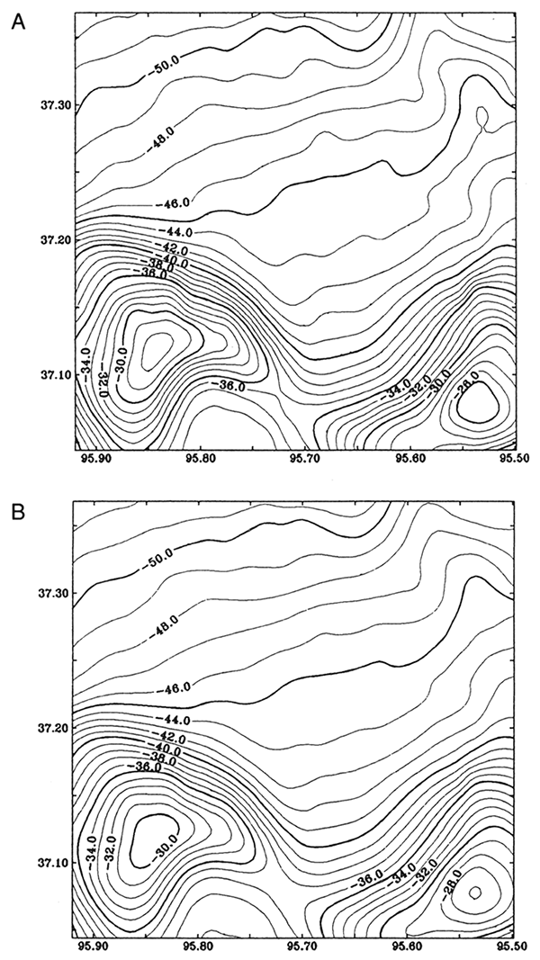
Gravity data were collected on the topographic surface with a spacing of 1.6 x 1.6 km (1 x 1 mi) in most of eastern Kansas and l.6 x 3.2 km (1 x 2 mi) in western Kansas. The data are available in the data base at Kansas Geological Survey (Lam and Yarger, 1989). The precision of the data is about 0.1 mGal. Figure 1A shows the Bouguer gravity map in Montgomery County. The first correction to the data is topographic (Xia and Sprowl, 1991) in order to reduce the data onto a horizontal plane. Figure 1B is a topographically corrected Bouguer anomaly map using a method discussed by Xia et al. (1991). After the correction, the data are on a horizontal plane of 700 m (2,297 ft) above sea level.
Figure 1--(A) Bouguer anomaly in Montgomery County, Kansas. Contour interval is 1 mGal. (B) Topographically corrected Bouguer anomaly on the level 700 m (2,297 ft) above sea level. Coordinates in figs. 1-15 are latitudes and longitudes.
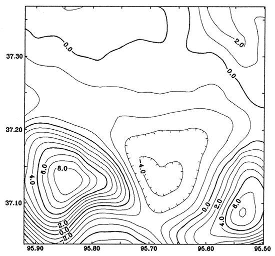
The second step of processing is to separate the anomaly. Abdelrahman et al.'s method (1985) is used to determine the optimum order of polynomial to separate the regional anomaly from the Bouguer anomaly. The overall similarity between each two successive residual maps was determined by calculating a correlation factor between the mapped variables. The correlation factors were computed using a formula given by Davis (1986, p. 40, Eq. 2.24, and p. 448). The lower order of two successive residual maps with the maximum value of the correlation factor was the optimum order of the polynomial to fit the regional surface. The correlation factor between the first-order and the second-order residuals is 0.9258, between the second-order and the third-order is 0.8102, and between the third-order and the fourth-order is 0.7468. Therefore, the optimum order of polynomial to fit the regional anomaly is 1. Figure 2 is the regional gravity map of the first-order polynomial trend, and fig. 3 is the residual Bouguer anomaly.
Figure 2--First-order polynomial represents the regional gravity anomaly. Contour interval is 1 mGal.
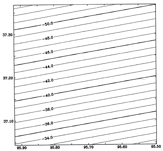
Figure 3--Residual gravity anomaly. Contour interval is 1 mGal.
Aeromagnetic data were collected with a flight-line spacing of 3.2 km (2 mi) and a tie-line spacing of 32 km (20 mi). In eastern Kansas the airplane was flown at a fixed elevation 762 m (2,500 ft) above sea level. In western Kansas the flight elevation was 915 m (3,002 ft) above sea level in the eastern portion and 1,372 m (4,502 ft) above sea level in the westernmost quarter of the state. The precision of the data is about 3 nT. Details of the data were described by Yarger (1983, 1989). Figure 4 is the aeromagnetic map in Montgomery County. The datum in the county is 762 m (2,500 ft) above sea level. For the magnetic data, one step of processing is needed: anomaly separation. The correlation factor between the first-order and second-order residuals is 0.9027, between the second-order and third-order is 0.9605, and between the third-order and fourth-order is 0.8945. Therefore, the optimum order of polynomial to fit the regional anomaly is 2. Figure 5 is the regional magnetic map of the second-order polynomial trend, and fig. 6 is the residual magnetic anomaly.
Figure 4--Aeromagnetic anomaly in Montgomery County, Kansas. Elevation of survey is 762 m (2,500 ft) above sea level; contour interval is 20 nT.
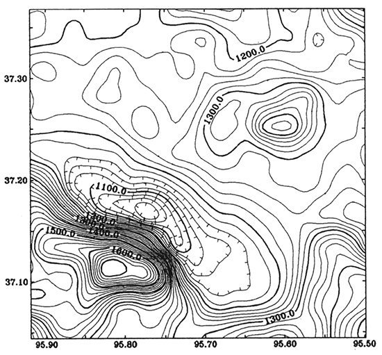
Figure 5--Second-order polynomial represents the regional magnetic anomaly. Contour interval is 20 nT.
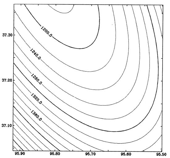
Figure 6--Residual magnetic anomaly. Contour interval is 20 nT.
In our study, all data are gridded into 24 x 23 matrix by SURFACE III (Sampson, 1988).
Based on the well data (fig. 7B), we calculated potential-field anomalies caused by the modified Precambrian subsurface terrane shown in fig. 7A. Assuming that the rocks of the Precambrian basement are mostly granitic, the average density of the basement was chosen as 2.70 g/cm3 (Garland, 1979). The rocks above the basement are shale, limestone, and sandstone, and the average density of these rocks is 2.43 g/cm3 (Garland, 1979) if the thickness of each is the same. Therefore, the density contrast of the interface would be 0.27 g/cm3 (= 2.70 - 2.43). We also assumed that the granitic rocks in the basement contained one percent of magnetite with the effective susceptibility K = 0.031 (SI units). Magnetization by the earth field of H = 40 A/m yields a magnetization of about 1.25 A/m (125 nT), which is an order-of-magnitude figure for polarization of basement rocks commonly used in magnetic-model calculations (Nettleton, 1976). Because sedimentary rocks are usually nonmagnetic, we used 125 nT as the magnetization in modeling the magnetic interface.
Figure 7--(A) Model of depth to the Precambrian basement. Contour interval is 50 ft (15 km). (B) Locations of the well data; units are in feet.
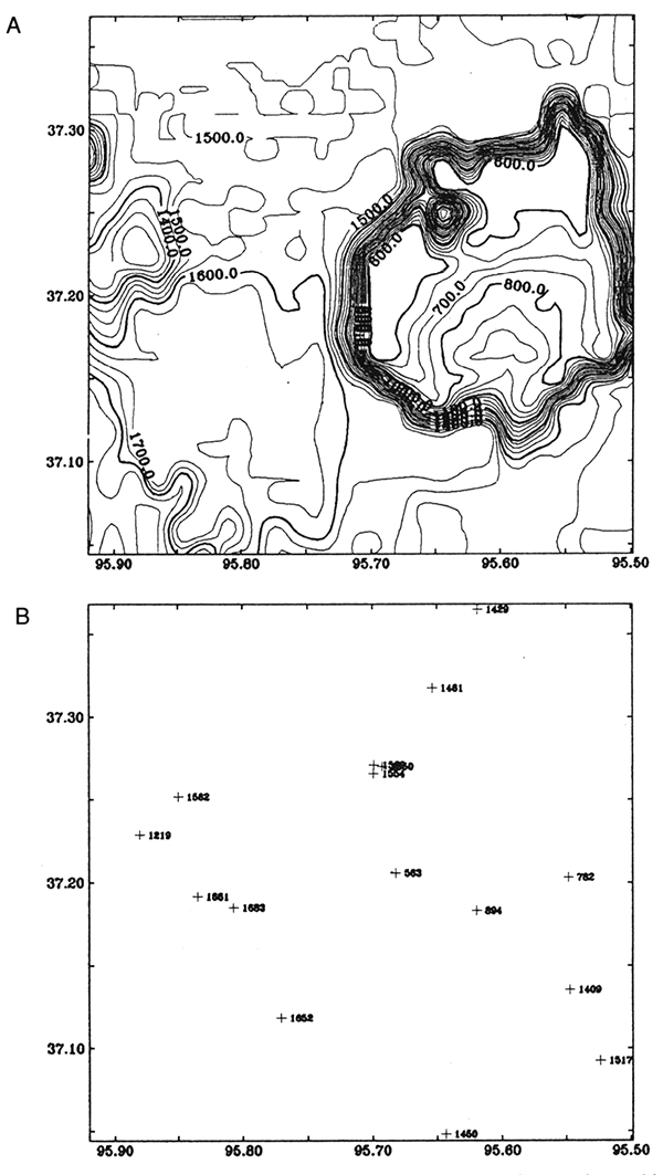
Figure 8 is the modeled gravity anomaly based on the basement model (fig. 7) with the density contrast of 0.27 g/cm3. Figure 9 is the modeled magnetic anomaly of the basement structure (fig. 7) with the magnetization of 125 nT. Parker's (1973) formula (Eq. 1) was used to calculate the anomalies. The inclination and declination of magnetization of the modeled magnetic anomaly are 65° and 7°, respectively, which are the direction of the normal earth field in Kansas. These modeled anomalies show that the main anomalies in the county are not caused by the Precambrian basement structure. The modeled anomalies (figs. 8 and 9) are subtracted from the residual gravity anomaly (fig. 3) and residual magnetic anomaly (fig. 6). Then we obtain remaining anomalies shown in figs. 10 and 11, respectively, which are assumed to have been caused by lithological changes in the basement. We try to invert the anomalies into density/ magnetization distribution in the basement.
Figure 8--Modeled gravity anomaly from the basement model (fig. 7A). Density contrast is 0.27 g/cm3. Contour interval is 0.2 mGal.
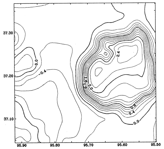
Figure 9--Modeled magnetic anomaly from the basement model (fig. 7A). Magnetization is 125 nT, and inclination and declination of the magnetization are 65° and 7°, respectively. Contour interval is 10 nT.
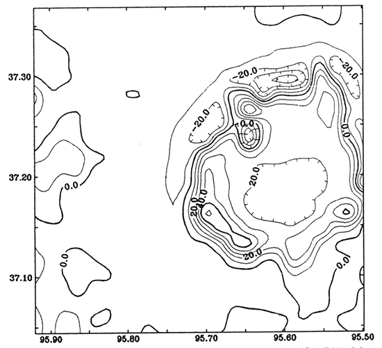
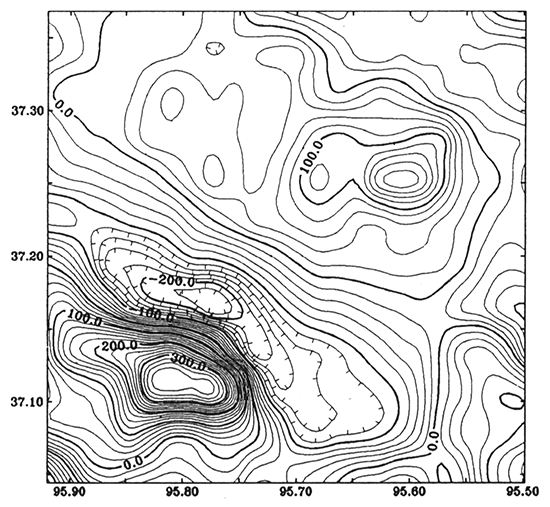
Figure 10--Gravity anomaly caused by lithological change in the basement, which is equal to the residual gravity anomaly (fig. 3) subtracting the modeled anomaly from the basement structure (fig 8). Contour interval is 1.0 mGal.
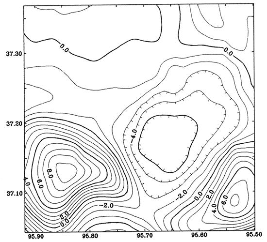
Figure 11--Magnetic anomaly caused by lithological change in the basement, which is equal to the residual magnetic anomaly (fig. 6) subtracting the modeled anomaly from the basement structure (fig. 9). Contour interval is 20 nT.

Xia and Sprowl's (1992) approach used in this study to invert the potential-field data is density/magnetization distribution within a layer. The computer program is described by Xia (1991). Calculation of a gravity anomaly field due to a material layer using Parker's formula (Eq. 1) requires three known functions: 1) the depth to the top of the layer (ZT = z1), 2) the depth to the bottom of the layer (ZB = Z2), and 3) the density distribution m:
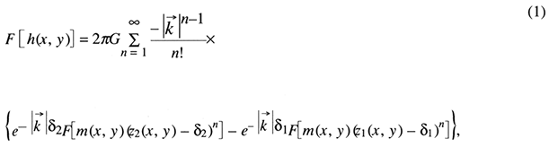
where G is the gravitational constant; ![]() is a wave number vector; δ1 and δ2 are the average value of z1 and z2, respectively; and F is the Fourier transformation. For calculating magnetic anomalies, the formula is little different from Eq. 1 and m is magnetization distribution, the direction of which must be known. The forward series expansion of Parker's formula is uniformly convergent for any reasonable topographic relief functions, ZT and ZB (Parker, 1973).
is a wave number vector; δ1 and δ2 are the average value of z1 and z2, respectively; and F is the Fourier transformation. For calculating magnetic anomalies, the formula is little different from Eq. 1 and m is magnetization distribution, the direction of which must be known. The forward series expansion of Parker's formula is uniformly convergent for any reasonable topographic relief functions, ZT and ZB (Parker, 1973).
Given ZT and ZB, the goal of inversion is to determine distribution function of density/magnetization m in the layer defined by ZT and ZB. The formulas that are used to modify the model after each iteration are listed below.
![]()
where superscript k stands for the kth iteration and subscript i for the ith data point; gi and hik are the measured and calculated gravity anomalies, respectively; G is the gravitational constant; and Δp is the density contrast.
![]()
where ZTik, the depth of ZT below point i at the kth iteration; hik and Ti are the calculated and measured total magnetic field anomalies, respectively; and ΔL is the average distance between data points, ΔJik is the modification to Jik, the magnetization below point i at the kth iteration.
Formula (2) is based on the Bouguer-slab formula. The formula (3) is simplified from the 2D vertical dike (Telford et al., 1982, p.166).
Two errors used to trace the iterative procedure are a root-mean-square error RMS(k) at the kth iteration:
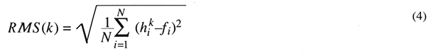
and the maximum deviation MAXD(k) at the kth iteration

where fi is the measured anomaly at the ith point, and N is the total number of data points. These two errors can tell the differences between a modeled anomaly and a real anomaly. At least, one of them should be reduced after each iteration in order to obtain stable convergence of the inverse procedure.
The inversion approach consists of three steps:
The uniqueness of the inverse model of density/magnetization distribution is restricted by the uncertainty in the functions ZT and ZB. Obviously, the thinner the layer is, the larger the value of density/magnetization. In our study, depth to the bottom of layer ZB in the inverse procedure is flexible. This uncertainty is reduced by known rock types on several well stations. The inverse models should be consistent with these well data. Actually, we choose several different depths for each anomaly to find an acceptable model in geology because the inverse model should honor the rock types shown by the well data. We found that 2,500 m (8,202 ft) below sea level for gravity inversion and 1,200 m (3,937 ft) below sea level for magnetic inversion are reasonable choices of ZB.
We invert fig. 10 (gravity anomaly caused by lithological change) into density distribution within the basement. The upper surface of the layer ZT is the basement and the bottom surface ZB is chosen as 2,500 m (8,202 ft) below sea level. The two surfaces are kept unchanged while solving for density distribution. We initialize the density 2.67 g/cm3, which is the average density of the continental crust. The initial RMS and DMAX errors are 11.4 mGal and 28.5 mGal, respectively. After 20 iterations, the errors RMS is reduced to 0.16 mGal and MAXD is reduced to 1.4 mGal. The final result, which represents the modified density distribution in the layer, is shown in fig. 12. The modeled gravity anomaly by lithological change is shown in fig. 13.
Figure 12--Inverse model from gravity anomaly (fig. 10): density distribution in the basement rocks. Mapping interval is 0.2 g/cm3.
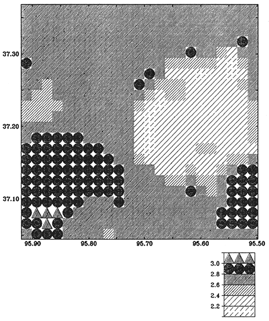
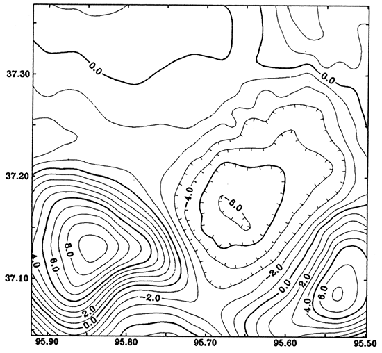
Figure 13--Modeled gravity anomaly from the inverse model (fig. 12). Contour interval is 1.0 mGal. The RMS and MAXD errors between figs. 10 and 13 are 0.16 mGal and 1.4 mGal, respectively.
We invert fig. 11 (magnetic anomaly caused by lithological change) into magnetization distribution. In this case, we define the upper surface of the layer ZT as the basement and the bottom ZB surface as 1,200 m (3,937 ft) below sea level. The two surfaces are kept unchanged while solving for magnetization distribution. The inclination and declination of the magnetization are 65° and 7°, respectively. We initialize magnetization 125 nT, which is the value of magnetization of the granitic rocks containing about 1% magnetite. RMS and MAXD of the initial model are 97.2 nT and 393.3 nt, respectively. After 33 iterations, RMS is reduced to 5.3 nT and MAXD is reduced to 18.8 nT. The final result, representing the modified magnetization distribution, is shown in fig. 14. The modeled magnetic anomaly by lithological change is shown in fig. 15.
Figure 14--Inverse model from magnetic anomaly (fig. 11); magnetization distribution in the basement rocks. Mapping interval is 100 nT.
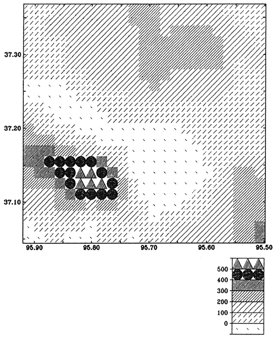
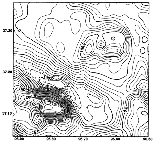
Figure 15--Modeled magnetic anomaly from the inverse model (fig. 14). Contour interval is 20 nT. The RMS and MAXD errors between figs. 11 and 14 are 5.3 nT and 18.8 nT, respectively.
Inverse procedure shows that two errors are reduced quickly and convergence of the iterations is stable. This shows that the formulas used to modify density/magnetization models work well.
Figures 12 and 14 show the inverse results. Density in most areas of fig. 12 is less than 2.80 g/cm3, but in the southeastern part density is above 2.80 g/cm3. According to Carmichael (1989, p. 163), densities greater than 2.80 g/cm3 will separate basalt from granite. In the same area of fig. 14, the magnetization is above 400 nT, which is about three times the content of magnetite (3%) in the rocks in this area as in the normal granitic basement. According to Carmichael (1989) and Nettleton (1976), the fact of higher density and higher magnetization in the area could be caused by basaltic rocks. However, Steeples and Bickford (1981) pointed out that the Miami County core, which is granite, contains about 2% of magnetite by weight. The source rocks, therefore, that cause the potential-field anomaly in southwestern Montgomery County are probably an intrusion of granodiorite containing more than 3% of magnetite.
Abdelrahman, E. M., Riad, S., Refai, E., and Amin, Y., 1985, On the least-squares residual anomaly determination: Geophysics, v. 50, p. 473-480
Cady, J. W., 1980, Calculation of gravity and magnetic anomalies of finite-length right polygonal prisms: Geophysics, v. 45, p. 1,507-1,512
Carmichael, R S. (ed.), 1989, Practical handbook of physical properties of rocks and minerals: CRC Press, Boca Raton, Florida, 741 p.
Davis, J. C., 1986, Statistics and data analysis in geology (2nd edition): New York, John Wiley & Sons, Inc., 646 p.
Dobrin, M. B., and Savit, C. H., 1988, Introduction to geophysical prospecting, 4th ed.: New York, McGraw-Hill, Inc., 867 p.
Garland, G. D., 1979, Introduction to geophysics--mantle, core, and crust: W. B. Saunders Company, 494 p.
Lam, C., and Yarger, H., 1989, State gravity map of Kansas: Kansas Geological Survey, Bulletin 226, p. 185-196 [available online]
Nettleton, L. L., 1976, Gravity and magnetics in oil prospecting: New York, McGraw-Hill Book Company, 464 p.
Parker, R. L., 1973, The rapid calculation of potential anomalies: Geophysical Journal of the Royal Astronomical Society, v. 31, p. 447-455
Plouff, D., 1976, Gravity and magnetic fields of polygonal prisms and application to magnetic terrain corrections: Geophysics, v. 41, p. 727-741
Sampson, R., 1988, SURFACE III: Lawrence, Kansas, Interactive Concepts, Inc.
Steeples, D. W., and Bickford, M. E., 1981, Piggyback drilling in Kansas--an example for the Continental Scientific Drilling Program: Transactions of the American Geophysical Union, v. 62, p. 473-476
Talwani, M., Worzel, J. L., and Landisman, M., 1959, Rapid gravity computations for two-dimensional bodies with application to the Mendocino submarine fracture zone: Journal of Geophysical Research, v. 64, p. 49-59
Telford, W. M., Geldart, L. P., Sheriff, R E., and Keys, D. A., 1976, Applied geophysics: Cambridge University Press, 859 p.
Xia, J., 1991, Computer program of inversion of potential-field data by iterative forward modeling: Kansas Geological Survey, Computer Program Series 91-2, 4 p., disk
Xia, J., and Sprowl, D. R., 1991, Correction of topographic distortions in gravity data: Geophysics, v. 56, p. 537-541
Xia, J., and Sprowl, D. R., 1992, Inversion of potential field data by iterative forward modeling in the wavenumber: Geophysics, v. 57, p. 126-130
Xia, J., Sprowl, D. R., and Adkins-Heljeson, D., 1991, A fast and accurate approach--correction of topographic distortions in potential-field data: Society of Exploration Geophysicists, 61st Annual Intemtational Meeting, Expanded Abstracts, p. 626-629
Yarger, H. L., 1983, Regional interpretation of Kansas aeromagnetic data: Kansas Geological Survey, Geophysics Series 1, 35 p. [available online]
Yarger, H. L., 1989, Major magnetic features in Kansas and their possible geologic significance: Kansas Geological Survey, Bulletin 226, p. 197-207 [available online]
Previous--Basement Control of Selected Oil and Gas Fields || Next--Midcontinent Rift System
Kansas Geological Survey
Comments to webadmin@kgs.ku.edu
Web version placed online Aug. 18, 2015. Original publication date 1995.
URL=http://www.kgs.ku.edu/Publications/Bulletins/237/Xia1/index.html