Kansas Geological Survey, Bulletin 109, pt. 7, originally published in 1954
Originally published in 1954 as Kansas Geological Survey Bulletin 109, pt. 7. This is, in general, the original text as published. The information has not been updated. An Acrobat PDF version (21.8 MB) is also available.
In order to investigate the application of resistivity methods to groundwater studies in eastern Kansas, electrical resistivity depth profiles were run in the Kansas River Valley at localities where geologic conditions were known. The results of this survey show that the depth to water table and bedrock can be determined in the Kansas River Valley. To a less certain degree interpretations can also be made concerning lithology and type of water contained in the alluvial sediments.
A series of preliminary electrical resistivity studies was made in the Kansas River Valley in eastern Kansas during 1953 (Pl. 1) in order to evaluate the possibilities of this geophysical prospecting method in the location of usable ground-water supplies. The Kansas River Valley was chosen for this preliminary study because of the abundance of available subsurface information. Test holes have been drilled by the State Geological Survey and by the U. S. Corps of Engineers to obtain information concerning ground water and bedrock. There are also numerous municipal, industrial, and domestic wells in this area from which information has been obtained. Furthermore, detailed geologic investigations of the ground-water resources recently have been completed by Davis and Carlson (1952) and Dufford (1953) and additional studies are under way by Henry V. Beck. As is true in the application of any geophysical method, the more geological data available, the better the interpretation of the results. In this area the resistivity profiles could be compared with known conditions of lithology, depth to water table, and depth to bedrock. These correlations then can be used to facilitate interpretation of profiles in areas which are geologically similar but lack well data.
Depth profiles were run at 33 places in the Kansas River Valley from Eudora to Belvue, Kansas, where test hole information was available.
The bedrock, Pennsylvanian in age, is overlain by Quaternary river alluvium. The alluvial fill attains a maximum thickness of 90 feet (Davis and Carlson, 1952, p. 229), but averages about 55 feet. The alluvial fill grades upward from a coarse cobble conglomerate in the deepest portions to fine sand or silt at the surface. The bedrock consists mainly of shale with some interbedded limestone and sandstone. The strata dip gently to the west from one-fourth to one-half a degree.
The saturated zone of water-bearing material ranges in thickness from about 20 to 65 feet (Davis and Carlson, 1952, p. 238). The depth to the water table ranges from about 5 to 30 feet from the surface. The quality of the ground water in the Kansas River Valley alluvium is good. Table 1 is a resume of chemical analyses as given by Davis and Carlson (1952, p. 245).
Table 1—Resume of chemical analyses of ground water from the Kansas River Valley alluvium. Dissolved constituents given in parts per million. [Note: One part per million is equivalent to one pound of substance per million pounds of water or 8.33 pounds per million gallons of water.] (Davis and Carlson, 1952, p. 245)
| Constituents | Minimum | Maximum |
|---|---|---|
| Dissolved solids | 346 | 828 |
| Silica | 2.4 | 38 |
| Iron | Trace | 13 |
| Calcium | 90 | 156 |
| Magnesium | 7.6 | 28 |
| Sodium and potassium | 16 | 174 |
| Sulfate | 4.5 | 106 |
| Chloride | 7 | 285 |
| Fluoride | 0.1 | 0.6 |
| Nitrate | 1.1 | 29 |
| Bicarbonate | 266 | 587 |
To my knowledge, no other work has been done on the uses of electrical-resistivity studies for the location of ground-water supplies in Kansas. Similar studies, however, have been conducted in other states, notably Illinois (Buhle, 1953).
Thanks are extended to Robert M. Dreyer, who suggested the problem and acquainted me with the field procedure and technique. Ralph E. O'Connor assisted with most of the field work and added many helpful suggestions. Many students at the University of Kansas and members of the State Geological Survey helped during various parts of the field work; these include Henry V. Beck, Donald O. Asquith, John C. Mann, and Robert O. Kulstad. John C. Frye made available unpublished manuscripts and other articles from his personal library and V. C. Fishel furnished unpublished ground-water information. R. M. Dreyer, M. B. Buhle, J. E. Hackett, and W. W. Hambleton read this report critically.
The resistivity equipment used is owned by the Department of Geology at the University of Kansas.
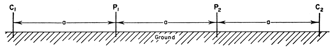
The instrument used was based on the Gish-Rooney circuit (Gish and Rooney, 1925), having a commutated direct current supplied from an external battery source. Four steel electrodes spaced equally distant in a straight line are placed in the ground from 6 to 12 inches deep (Pl. 2A). A measurable current is passed through the ground by way of the two outer electrodes and the potential drop is measured between the two inner electrodes. The two energizing electrodes are placed on the outside of the potential electrodes. This symmetrical arrangement with an equal spacing of the electrodes is known as the Wenner (Wenner, 1916) electrode configuration (Fig. 1).
Plate 2—A, Set-up of resistivity equipment in field operation. B, Electrical resistivity instrument and the logging device. (Photo by Ada Swineford)
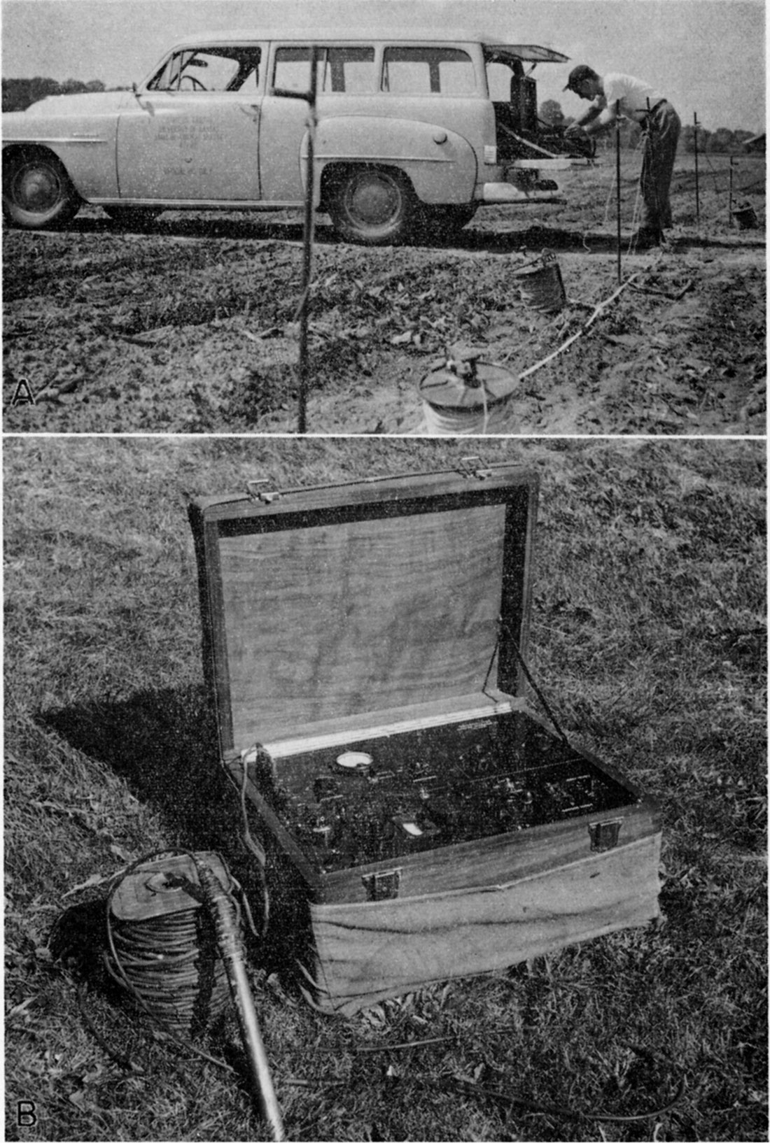
Figure 1—Schematic diagram showing the Wenner electrode configuration. C1 and C2 are the current electrodes; P1 and P2 are the potential electrodes; a is the distance between them. As a increases the depth of penetration also increases.
The effective depth to which the specific resistance to flow of an electric current is measured is dependent upon the spacing of the electrodes and the resistivity of the materials through which the current passes. When the electrodes are placed in the ground at equal spacings in a straight line, the effective depth penetration in homogeneous material is theoretically one-third the total spread or equal to the distance of the spacing of the two inner or potential electrodes. However, since the materials measured generally are not homogeneous, the depth of penetration will change from place to place and must be determined empirically for each new area.
Two types of resistivity measurements may be made: (1) vertical and (2) lateral. The vertical profiles are constructed by progressively increasing the distance between the electrodes as they are moved out from a common center. Lateral investigations are made by taking a single reading at each of several stations along a traverse line, maintaining a constant electrode spread and moving the entire configuration. The purpose of lateral investigation is to detect horizontal changes. Both methods are applicable to groundwater studies depending upon the results desired; however, only vertical investigations were used in this study.
Relatively flat ground was selected for each survey to eliminate the necessity of topographic corrections. No more than a 2-foot difference in elevation occurred at anyone station. Extreme care was taken to avoid power lines, steel fences, buried pipe lines, cased wells, and culverts which might act as shunts or otherwise disturb the electrical system. For this reason no profiles were run inside any town. Open ditches, such as irrigation ditches, also were avoided. Most of the profiles were run in a north-south direction which is roughly normal to the trend of the valley. However, when profiles were run in an east-west direction because it was impossible to spread the electrodes north-south, no appreciable differences were found. The depth profiles were run as near as possible to the wells for which records were available. From one to five men were used. An ideal crew for extensive work would contain six—one man to move each electrode, an instrument man, and a computer.
Usually readings were started at a depth of 5 feet and taken every 2 or 3 feet until the water table was reached and then at 5-foot intervals into bedrock. Each reading was then computed and plotted for interpretation.
The computations are based on the principle of Ohm's law: R = V/I (where R = resistance, V = voltage, and I = current). By using a known current and measuring the voltage, it is possible to compute the average rock resistivity within the zone of measurement. When the Wenner configuration is used, the formula, which is a derivation of Ohm's law, for computing the apparent resistivity is:
p = 2πa V/I
(where p = resistivity in ohm-feet, a = the distance between the electrodes in feet, V = the voltage in volts, and I = the current in amperes).
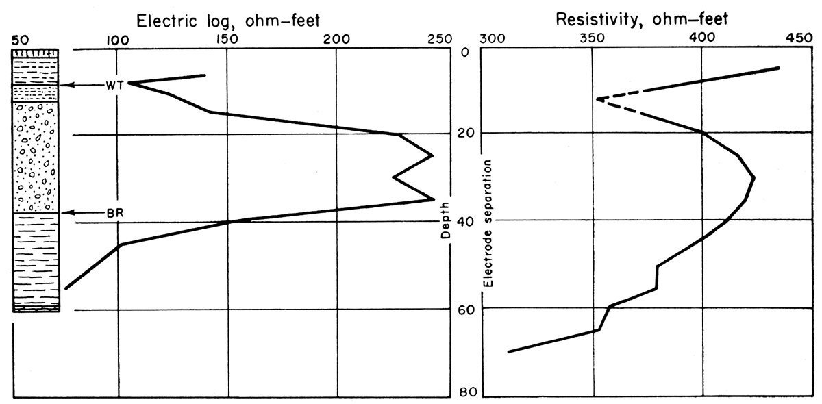
There are several methods by which resistivity data can be interpreted. In this report interpretations are based on a visual comparison of resistivity data with geologic data from well logs. To help with the interpretations, an electric log was run on test hole R-7 for comparison with the depth profile obtained at the same location (Fig. 2). An electric log was run immediately after the well was drilled, with a logging device which is attachable to the resistivity instruments (Pl. 2B) . This log shows that the resistivity decreases until the water table is reached, increases sharply until bedrock is reached, and then decreases again. It will be noted that the interpretation of the water table, as shown on the well log, corresponds to a lithologic change from silt and clay to sand. In general, the apparent resistivity of a lithologic unit in an electric well log is a function of the ionic content of water in the given strata. If the water has become mineralized in a particular strata the resistance of that bed will be low. The resistivity curve then may show the contrast between the contained waters of two beds of unlike lithology. The resistivity depth profiles may be interpreted in the same manner as interpretations made from the electric log.
Figure 2—Comparison of an electric log with a resistivity depth profile. Shows by visual comparison the relationships between the electric log and a depth profile and the lithologic log at the test hole R-7. WT is the measured depth to the water table and BR is the measured depth to bedrock.
There are four items which might be determined from these resistivity profiles in the Kansas River Valley: (1) depth to water table, (2) depth to bedrock, (3) type of lithology, and (4) type of water. The last two are more difficult to interpret than the first two.
As most of the wells had been drilled several years before the resistivity surveys were run, the present depth to the water table could not be obtained. However, a few of the holes were still open and the depth to the water table could be measured.
Generally the resistivity of the material decreases until the water table is reached and then it increases. However, in some of the profiles the opposite was found. This latter situation is interpreted to mean that the water is mineralized with a high ion content. Some of the profiles do not show a change of resistivity at the water table. Most curves were run very close to Kansas River on low ground in wet weather and it is probable that the water 'table was very near the surface. Water-table determinations could not be made on other profiles which were logged as dry holes.
The bedrock contact is relatively easy to determine because the resistivity of the bedrock is usually less than that of the water-filled alluvium. However, some of the profiles are straight and featureless, showing little contrast in resistivity of the alluvium and the bedrock. This is especially true where either dry alluvium or alluvial silt and clay were found to overlie bedrock of weathered shale. In some profiles the resistivity of the water-filled alluvium was so high that it almost completely masked the bedrock contact.
Lithology can be interpreted to a limited extent from an examination of the configuration of the curves. As alluvium, in general, has a higher resistivity than the bedrock the curves show more irregularities due to local lithologic variations. In general, sand and gravel have a higher resistivity than silt and clay. Profiles that show relatively high resistivity probably indicate fresh water, whereas the profiles showing relatively low resistivity probably indicate mineralized water. According to Heiland (1937, p. 574), water with a resistivity of less than 440 ohm-feet (1350 ohm-cm) should be avoided for human use, and down to about 165 ohm-feet (500 ohm-cm) is tolerable for stock use. Salinity interpretations, however, are uncertain other than for the two extremes—fresh or brackish. Since no brackish water occurs in this area, salinity determinations were not possible.
The comparison of the depth profiles and the well logs is shown on Plate 1. The water table as interpreted from the resistivity profiles is marked by a "WT" and the bedrock contact by a "BR."
Moore's (1945, p. 197) cumulative method of interpretation was applied to the profiles and found to be a satisfactory method of determining bedrock. Although the validity of the method is questioned by some, it seems to give excellent results in aiding interpretations of profiles in the Kansas River Valley. Only a few of the profiles could not be analyzed by this method.
Profiles E-1 and E-2 show an increase in resistivity until the water table is reached and then a decrease. This decrease in resistivity possibly is due to a lens of mineralized water between 25 and 50 feet. The bedrock contact in these two profiles does not show a sharp decrease in the electrical resistivity, but rather a gentle break in the curve caused by slightly increased resistivity. Profile E-3 shows little form with an over-all low resistivity. The water table in this profile occurs in a clay bed in contrast to E-1 and E-2 where the water table occurs approximately at the top of the sand.
Profiles L-1, L-2, and L-3 show similar characteristics. The resistivity decreases to the water table and then increases until bedrock is reached. The bedrock in all three profiles is sandstone. The irregularity of the resistivity curves in bedrock below the alluvium possibly can be attributed to a sequence of alternating sandstone and shale beds.
Profile LV-1 was logged as a dry hole and thus shows no water-table break on the curve. The straightness, lack of feature, and gradual increase in resistivity with depth seem to be characteristic of alluvial material which lacks water saturation. Profile LV-2 shows a high resistivity between 20 and 40 feet which probably indicates fresh water in that interval. The drillers logs at LV-3 and LV-4 found bedrock at 51 and 52 feet respectively, whereas the resistivity profiles could be interpreted as showing bedrock at 80 and 75 feet respectively. This discrepancy can be explained in two ways: (1) the limestone and shale, logged as bedrock by the driller, are boulders in the alluvial fill and thus not bedrock or (2) the interpretation of the resistivity profiles is in error because of some anomalous electrical property of the material in this area. It has been found, in certain areas, that a silt bed, such as the one here, will completely mask the electrical properties of the lower beds (Buhle, personal communication) . The profile LV-5 is unusual because it shows a gradual decrease of resistivity with depth into bedrock. On the electrical resistivity profile, bedrock is placed tentatively where the rate of decrease in resistivity becomes less.
Profile P-1 is unusual because of the sharp breaks of the curve. P-2 shows a high resistivity between 15 and 30 feet which is probably fresh water. The bedrock contact, as logged in the test well, does not compare favorably with the resistivity curve in profile P-3. Possibly some near-surface anomaly is masking the electrical properties of the lower beds. Profile P-4 shows a more characteristic type of curve with the drillers log and resistivity curve in close agreement.
All three of the resistivity curves show a good break at the water table. Bedrock could not be interpreted from profile T-1. Profiles T-2 and T-3 show more characteristic curves. The increased resistivity between 20 and 40 feet on profile T-3 could be interpreted as a lens of fresh water in that interval.
Profiles K-1, K-2, and K-3 show good breaks at the water table. The discrepancy in the interpretation of bedrock in profiles K-1 and K-2 possibly is due to the fact that the shale logged as bedrock is actually part of the alluvium.
Profiles SL-3, SL-4, and SL-5 show a high resistivity for the sand and gravel beds of the alluvium which tend to indicate that they probably contain fresh water. Bedrock in the profiles is marked by a decrease in resistivity. These curves are good illustrations of a fresh water-bearing alluvium overlying a bedrock shale sequence. The profiles SL-5 and SL-6, show good water-table breaks.
Profile R-5 does not show an interpretable break either at the water table or at bedrock. The lack of features on this curve may be due to the masking effect of the overlying near-surface clay bed. Profile R-6 shows an overall decrease in resistivity with depth. Profiles R-6, R-7, R-8, and R-9 show good water-table breaks. Profile R-9 might be termed an ideally shaped curve.
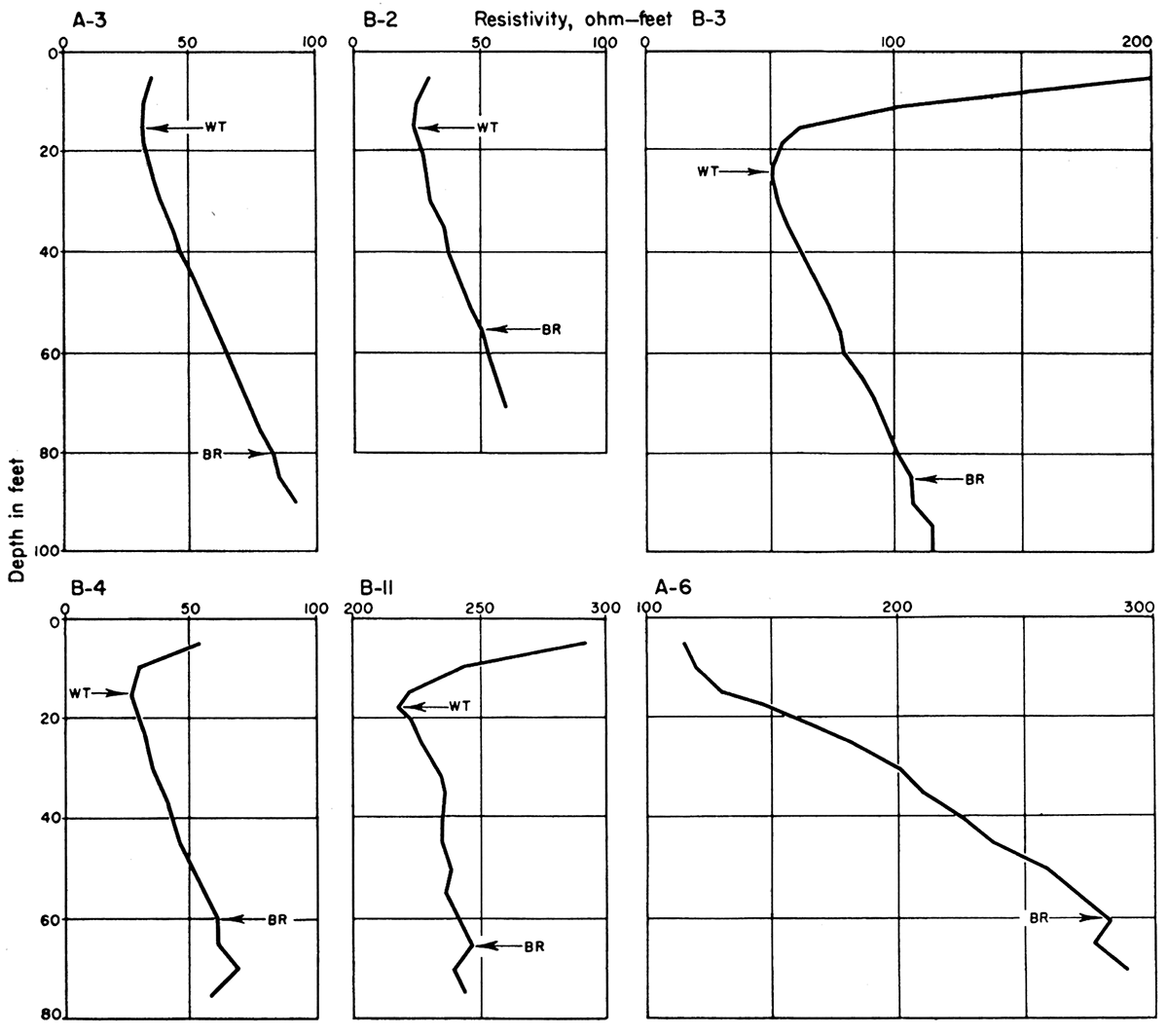
The profiles at B-1 and B-2 are similar in shape and configuration. The two curves show an over-all increase in resistivity into bedrock. However, a slight break in rate of increase of resistivity is interpreted as bedrock on both profiles. The high resistivity shown on profile B-3 is probably due to fresh water in the alluvial sand.
The average error in picking the water table is about 15 percent, whereas the error in interpretation of bedrock is only 9 percent. With a refinement of technique this percentage of error probably could be reduced. Table 2 is a resume of the water-table measurements and those obtained by resistivity methods. Generally, the water table can be determined within 2 feet when using a 2-foot interval spread in taking the depth measurements. The best results in locating the water table seem to be obtained when it is 15 feet or more below the surface. Table 3 is a resume of bedrock as determined by drilling and by resistivity methods. Using a 5-foot interval in taking depth measurements, the bedrock usually can be determined within 5 feet.
Table 2—Water-table measurements compared with resistivity findings
| Profile number | Water table by direct measurement, feet |
Water table by resistivity, feet |
|---|---|---|
| E-1 | 20 1/2 | 20 |
| E-2 | 20 | 15 |
| P-1 | 3 | 5 or less |
| B-1 | 17 | 12 |
| B-2 | 21 | 15 |
| R-7 | 6 | 8 |
| R-8 | 17 | 16 |
| R-9 | 17 | 15 |
| SL-4 | 7 1/2 | 5 or less |
| SL-5 | 17 | 15 |
| SL-6 | 14 | 12 |
Table 3—Bedrock as determined by drilling compared with bedrock as determined by resistivity methods
| Profile number | Bedrock as determined by drilling, feet |
Bedrock as determined by resistivity, feet |
|---|---|---|
| E-1 | 55 | 50 |
| E-2 | 65 | 55 |
| E-3 | 76 | 80 |
| L-1 | 79 | 70 |
| L-2 | 60 | 55 |
| L-3 | 42 | 40 |
| P-1 | 48 | 50 |
| P-2 | 41 | 40 |
| P-3 | 47 | 60 |
| P-4 | 75 | 80 |
| T-2 | 79 | 90 |
| T-3 | 49 | 50 |
| K-1 | 65 | 70 |
| K-2 | 72 | 65 |
| K-3 | 75 | 75 |
| B-2 | 78 | 75 |
| B-3 | 50 | 50 |
| R-6 | 41 | 45 |
| R-7 | 38 | 50 |
| R-8 | 65 | 65 |
| R-9 | 50 | 55 |
| SL-3 | 74 | 65 |
| SL-4 | 65 | 70 |
| SL-5 | 74 1/2 | 75 |
| SL-6 | 49 | 60 |
| LV-1 | 53 | 60 |
| LV-2 | 68 | 55 |
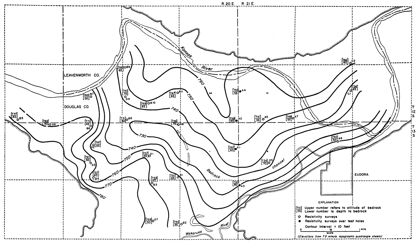
The information obtained from the resistivity profiles at the location of the test holes was utilized in a small area in the Kansas River Valley between Lawrence and Eudora for the construction of contours showing the configuration of the water table and the bedrock surface. Interpretations of water table and bedrock from profiles in this area were determined by visual comparison of curves obtained at the location of test holes in the vicinity. Some of the representative resistivity profiles are presented in Figure 3. The depths to water table and bedrock were computed to sea level, plotted, and then contoured. Figure 4 shows-the configuration of the top of the water table. Information from both the resistivity surveys and direct measurements were used. This map shows a remarkable similarity to a water-table map prepared by Dufford (1953, pl. 3) on information obtained only from test holes and water wells. With the stations spaced even closer together, a more detailed map could be obtained. The configuration of the bedrock as determined from the resistivity profiles is shown in Figure 5. The most significant feature on this map is an old bedrock river channel below the alluvium.
Figure 3—Representative resistivity profiles in the Lawrence-Eudora area. WT marks the water table as interpreted from the resistivity profile and BR marks the bedrock contact as interpreted from the resistivity profile,
Electrical resistivity methods have been shown to be an effective way of prospecting for ground water and for mapping alluvium-bedrock contacts in the Kansas River Valley. Within limits, the depth to the water table and to bedrock can be determined. Some information also can be obtained concerning the lithology of the materials and type of ground water they contain. The full utilization of this method has not yet been recognized and should be tried at other pertinent localities in Kansas.
Figure 4—Configuration on top of the water table in the Lawrence-Eudora area. Information from resistivity surveys and actual measurements shows the mounding effect of the water table between Kansas River and Wakarusa River.
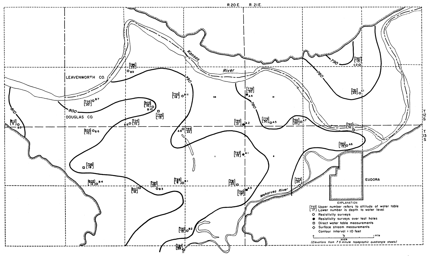
Figure 5—Configuration of the bedrock in the Lawrence-Eudora area. Information from resistivity surveys and actual measurements shows the configuration on top of the bedrock. A bedrock channel (along with several minor tributaries to the main channel) is outlined below the river alluvium.
Buhle, M. B. (1953) Earth resistivity in groundwater studies in Illinois: Am. Inst. Mining and Met. Engineers Trans., Tech. Paper 3496L, Mining Engineering, April, pp. 395-399.
Davis, S. N., and Carlson, W. A. (1952) Geology and ground-water resources of the Kansas River Valley between Lawrence and Topeka, Kansas: Kansas Geol. Survey, Bull. 96, pt. 5, pp. 201-276. [available online]
Dufford, A. E. (1953) Quaternary geology and ground-water resources of Kansas River Valley between Bonner Springs and Lawrence, Kansas: unpublished master's thesis, University of Kansas Library,
Gish, O. E., and Rooney, W. J. (1925) Measurement of resistivity of large masses of undisturbed earth: Terrestrial Magnetism, vol. 30, pp, 161-188,
Heiland, C. A. (1937) Prospecting for water with geophysical methods: Am. Geophys. Union Trans., pt. 2, pp. 574-588.
Lohman, S. W. (1941) Ground-water conditions in the vicinity of Lawrence, Kansas: Kansas Geol. Survey, Bull. 38, pt. 2, pp. 17-64. [available online]
Moore, R. W. (1945) An empirical method of interpretation of earth-resistivity measurements: Am. Inst. Mining and Met. Engineers Trans., vol. 164 (Geophysics), pp. 197-214.
Wenner, Frank (1916) A method of measuring resistivity in the earth: U. S. Bur. Standards, Bull. 12, pp. 469-478.
Wyman, Theodore (1935) Report on Kansas River, Kansas, Colorado, and Nebraska: 73d Congress, 2d Sess., House Doc. 195, pp. 1-331.
Kansas Geological Survey
Placed on web Jan. 2, 2019; originally published Oct. 15, 1954.
Comments to webadmin@kgs.ku.edu
The URL for this page is http://www.kgs.ku.edu/Publications/Bulletins/109_7/index.html