Kansas Geological Survey, Open-file Report 2015-1
Kansas Water Office Contract 13-0114 & 14-104
KGS Open File Report 2015-1
February 2015
The complete report is available as an Adobe Acrobat PDF file (3 MB).
The Republican River Basin encompasses approximately 24,540 square miles of eastern Colorado, southern Nebraska, and northern Kansas that drain to the Republican River above the gaging station at Clay Center, Kansas (fig. 1). The study area contains more than 2.7 million acres of irrigated agriculture served by a combination of surface and groundwater supplies. Of these, 1.6 million acres are in Nebraska, 435,000 acres are in Kansas, and 550,000 acres are in Colorado. In addition to irrigated agriculture, the water resources serve municipalities, industry, recreation, and wildlife.
Figure 1--Location of the Republican River Basin, including sub-basins. Study area, here referred to as the Lower Republican River Basin, is shaded grey. Hatched area denotes location underlain by the High Plains Aquifer.
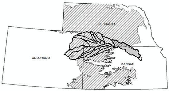
The entire study area includes seven U.S. Bureau of Reclamation (USBR) storage reservoirs, one U.S. Army Corps of Engineers reservoir (Harlan County Lake [HCL]), and two irrigation canal districts that supply water to agriculture. Much of the upper basin is underlain by the High Plains aquifer, which is used extensively for irrigation purposes. Alluvial aquifers are also present along the Republican River itself, and these aquifers are used for irrigation throughout the basin. Because of long-term imbalances between water supply and demand, Colorado, Nebraska, and Kansas ratified an interstate compact in 1943 to ensure equitable distribution of water within the basin. The compact also dictates that each state must efficiently manage its resources and should continuously try to improve efficiency measures to address current and future water supply issues. This project aims to improve the water management within the basin, focusing on the Lower Republican River Basin (LRRB) in Kansas.
The KWO contracted with the Kansas Geological Survey (KGS) in the fall of 2012 to develop a numerical groundwater/surface water model of the LRRB as a component of a larger project (the Republican River Basin Study) administered by the USBR through a WaterSMART Basin Study. The overarching objective of the Republican River Basin Study is to formulate and evaluate alternative solutions to address current and future water-supply issues within a basin-wide framework. The LRRB study focuses on the region between the HCL outflow and the inlet to Milford Reservoir (fig. 2).
The objectives of the overall study are to estimate current and future water supplies and demands in the Republican River Basin and to assess the effects of projected future climates on water resources, water management and water rights, and natural and ecological needs. Transparent and scientifically defensible hydrologic modeling tools are being developed to aid in conjunctive surface water/groundwater management planning. These tools will be used to assess system performance and evaluate structural and operational management alternatives under current and projected water supply and demand conditions in support of integrated surface water and groundwater management planning in the basin. Based upon these assessments, recommendations will be made for structural and operational alternatives to optimize surface water and groundwater use in the basin and address current and future water supply imbalances.
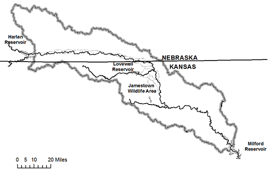
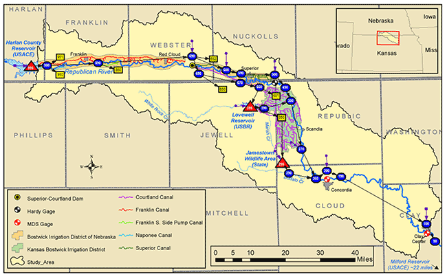
The focus of this work is on the LRRB in Kansas (fig. 1), covering 4,000 mi2 and extending from the outlet of HCL to the inlet of Milford Reservoir (fig. 2). This area contains two reservoirs (HCL and Lovewell) and both of the irrigation canal districts. The LRRB in Kansas is not underlain by the High Plains aquifer; subsurface resources are derived almost entirely from the alluvial aquifer along the Republican River channel.
This open-file report (OFR) documents the development and calibration of the LRRB surface/subsurface hydrologic model produced as part of this study. In addition to the linkage to the surface water operations model used in the study, it also briefly describes the water-routing program OASIS, or Operational Analysis and Simulation of Integrated Systems. This OFR does not describe the development of the OASIS LRRB model or simulation results of future climate or alternative management scenarios.
As part of the larger Republican River Basin study administered by the USBR, members of the study group and the USBR oversaw the model development. The technical group involved in the USBR study had biweekly conference calls, and the Kansas technical team met and interacted on a more frequent basis. As part of the USBR study, study partners developed and reviewed technical memoranda, which then served as the basis for the study report.
The USBR study also included stakeholder group and public meetings to discuss goals, objectives, and results of the study. The Kansas team met with the Lower Republican River Management Advisory Committee in November 2013 and in March 2014 to present ongoing model results. In addition, the model development was presented at the 2014 Midwest Groundwater Conference, 2014 NGWA Groundwater Summit, 2014 AEG Kansas Hydrology Seminar, 2013 and 2012 Governor's Conference on the Future of Water in Kansas, 2013 HGS User's meeting, and 2012 GSA annual meeting.
The study area includes the LRRB and extends from the HCL outlet in Nebraska to the Milford Reservoir inlet (fig. 2). The total area covered by the model is 4,000 square miles.
Figure 2--Lower Republican River Basin study area. Republican River and main tributaries are represented by black lines and primary irrigation canals by gray lines.
The model area lies within the physiographic provinces of High Plains, Smoky Hills, and Flint Hills Upland within the greater Great Plains physiographic province. The geologic properties are generally characterized by the exposure of limestone, shale, and sandstone of the Cretaceous and Permian age, with a trend of progressively younger rocks exposed from east to west. The sand and gravel alluvium found in the valleys are the primary source of groundwater in this region (Sophocleous et al., 1997).
The LRRB has been the topic of many research studies, stemming from both the administration of the interstate compact and from the desire of Kansas, Nebraska, and Colorado to improve water-use efficiency within their borders. Past studies include several open-file reports from the Kansas Geological Survey (KGS), including stream/aquifer studies and model development (Sophocleous et al., 1995; Sophocleous et al., 1997; Perkins and Sophocleous, 1997). More recent studies include the development of the Republican River Compact Model (RRCM), which simulates the baseflow component of the Republican River to evaluate the effects of groundwater pumping and recharge on river water quantities (Republican River Compact Administration, 2003). The RRCM only extends to the Kansas-Nebraska border and thus does not include the entire LRRB domain. The State of Kansas was part of an appraisal study in 2005 with Nebraska to evaluate alternatives for more efficient water management as part of the USBR WaterSMART program. That study, which synthesized existing data and did not collect any additional field data, determined that some water supplies in the LRRB are not being fully utilized. With improvements in the existing systems and with increased storage capacities, the system could be better managed to alleviate some of the water shortage problems and provide some streamflow augmentation in the lower reaches in Kansas. These system improvements include converting open-ditch laterals into buried pipes, automating the Courtland Canal system to allow for off-season diversions, and increasing storage of the Lovewell Reservoir (Nebraska and Kansas, 2005). These system improvements will be simulated as part of this research effort.
The model development presented here is part of a feasibility study being conducted on the Republican River Basin as part of the USBR WaterSMART program. This study includes scientists from Colorado, Nebraska, and Kansas in addition to the USBR. The objective of this study is to evaluate water- management strategies, including some from the Appraisal Report (Nebraska and Kansas, 2005), to determine the most efficient method for meeting future water demands under predicted changes to future climate.
HydroGeoSphere
The integrated surface water/groundwater hydrologic model developed in this project was constructed using HydroGeoSphere (HGS; Therrien et al., 2007). Fully integrated surface/subsurface hydrologic models can incorporate the details of both the surface and subsurface flow regimes and can capture and quantify all groundwater/surface water interactions. Developed by researchers at the University of Waterloo, HydroGeoSphere is capable of simulating two-dimensional depth-integrated overland/stream flow and transport and three-dimensional variably saturated flow and transport in the subsurface. It is also capable of simulating the effects of pumping wells and spatially and temporally variable evapotranspiration, both of which are important components of the LRRB hydrologic system. The surface/subsurface flow and transport equations are solved using a globally implicit Control-Volume Finite Element method (Therrien et al., 2007).
OASIS
A water routing program, OASIS (Operational Analysis and Simulation of Integrated Systems), was used to account for surface water operations governing reservoir, canal, and river management in the basin (Hydrologics, 2009). The OASIS model simulates the routing of water through a system, while accounting for both physical and operational constraints on a system. Physical constraints can include inflows to the reservoirs, reservoir evaporation, streamflows, reservoir sedimentation, and routing of water through the system. Operational constraints (or system-management issues) include reservoir minimum-release requirements, water-user demands, lake-level management plans, and operations agreements. The OASIS model improves upon traditional spreadsheet models because it simulates the interaction of multiple reservoirs and rivers in a system, improves the ability to simulate system- management issues, and identifies problematic areas in a system. The OASIS models were initially developed by Hydrologics, Inc. and consist of a system of nodes that represent reservoirs and demands, arcs that represent river reaches, historical data that can be used to project future basin conditions, and operational control language (OCL). OCL can be created to simulate any physical or operational constraint that may apply to a system, such as lake release schedules and criteria, a water right's relative priority to the lakes' water reservation right priority, or target flows at specified points on the stream.
HGS-OASIS Linkage
The hydrologic system as simulated by HGS and the surface water operations as simulated by OASIS are part of the same larger hydrologic environment. Reservoir releases strongly influence river water levels and, hence, groundwater/surface water interactions. Conversely, temporal and/or spatial variations in gains or losses along the river channel can influence the timing and quantity of water released from reservoirs. As such, HGS and OASIS were linked as part of this work to represent the system holistically. Changes were made to both codes to allow information to be passed between them automatically throughout the simulations. This allows the natural hydrologic system to respond to surface water operations and to provide feedback to water-management operations of groundwater/surface water interactions throughout the domain.
OASIS OCL was developed to write output files formatted for HGS. Three output files are written from OASIS at each time step: reservoir releases, irrigation district demands, and Minimum Desirable Streamflow (MDS) administration.
Reservoir Releases
Reservoir releases are calculated within OASIS and are converted to m3/s and written to a file formatted for HGS. Within HGS, these values are input as a nodal flux boundary condition (which uses volumetric fluxes) at the node located closest to the reservoir outlet. As the Lovewell Reservoir is located entirely within the bounds of the HGS domain, this water must also be removed from a portion of the domain to conserve mass. The reservoir volumes are not defined with HGS. However the Digital Elevation Model (DEM) was altered to reflect an estimate of the reservoir bottom, allowing water to pool in the nodes that represent the reservoir. The water released from Lovewell Reservoir is taken from all the reservoir nodes equally. This was achieved through the development of the flux multiplier feature in HGS. This feature allows the user to designate a multiplier to be applied to selected flux boundary conditions. For the Lovewell Reservoir, a multiplier of -0.33 is applied to the reservoir release value output from OASIS for each of the three reservoir nodes. This allows HGS to use the same OASIS output file for both removing water from the reservoir and entering it into the stream system.
The Jamestown Wildlife Area does not currently operate as a reservoir. Thus, water is simply routed through this region.
Irrigation District Demands
Demands from the irrigation districts were also calculated within OASIS before linking to HGS. Similar to the reservoir release data, values were converted to m3/s and written to a file formatted for HGS. To conserve mass, this water must be taken from the stream system and applied as irrigation to the associated upland areas. The demands are written as negative values by OASIS and are read as volumetric fluxes at the node located closest to the water right along the main stem of the river system in HGS. This removes water from the stream in a location where there will be enough water to satisfy the demand. Given the topographical resolution of the HGS model, routing of water from the main stem through smaller tributaries and canal systems is not captured. The flux multiplier feature is used to distribute the water as irrigation return flow to a group of 20 nodes within the irrigation district that called for the water release.
Minimum Desirable Streamflow Administration
Minimum Desirable Streamflow (MDS) requirements are part of the Kansas Water Appropriation Act by the Kansas Legislature to "ensure baseflow conditions in certain streams to protect existing water rights and to meet in-stream water uses related to water quality, fish and wildlife and recreation" (www.agriculture.ks.gov). When MDS is administered, water rights junior to the MDS administration date (April 12, 1984) are closed until the MDS is no longer administered.
OASIS passes MDS administration to HGS as a binary number: 0 when MDS administration is applied to junior wells and 1 when it is not. HGS was developed to administer MDS to a selection of fluxes representing the water rights junior to the MDS. These fluxes are multiplied by the binary number passed by OASIS, and thus are turned off when MDS is administered. During the calibration period, this function was not used.
Stream Gains/Losses
HGS code was also written to calculate and pass the stream segment gains/losses to OASIS. A feature was programmed to write data for input into OASIS for a designated number of segments within the domain. The user must provide a file for each segment listing the HGS node numbers associated with the segment. HGS multiplies each nodal exchange flux between the groundwater and surface water (m/s) by the area represented by the node and adds all nodal volumes together to get a total volumetric gain or loss through the segment to pass to OASIS.
OCL was written in OASIS to read the HGS output of gains/losses (m3/s) of stream segments for each time step. These gains/losses are input to the model at predetermined nodes within OASIS and represent the reach gains/losses between the previous input node and the current node.
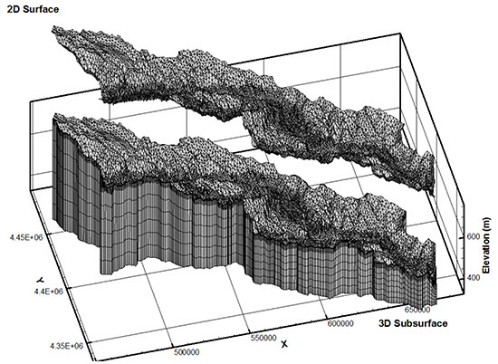
The HGS model domain was discretized using prism elements of variable sizes. Each layer includes 17,591 elements (9,032 nodes), and the subsurface is divided into 15 layers varying between 1 m and 20 m in thickness (distance between layers increases with depth) (fig. 3). A 2D triangular mesh that maps directly onto corresponding nodes in the subsurface represents the surface flow domain (fig. 3). The surface elevation of the model was mapped using a 30-m Data Elevation Model (DEM) from the National Elevation Dataset created by the USGS EROS Data Center, and the bottom boundary is located at 250 masl, suitably deep to not affect the areas of interest in this study. Lateral edges of the domain follow the regional surface water divide.
Model development was divided into three phases for this study. First, a steady-state simulation that represented the predevelopment period (pre-1950) was developed for HGS. During this period, no groundwater or surface water pumping activities were present in the model. Second, a transient simulation was conducted for a calibration period between 1950 and 1990 and validation between 1990 and 2010 to simulate the historic development of the groundwater and surface water system of the LRRB. The calibration period was split into two sub-steps: from 1950 to 1990, for which HGS and OASIS were operated independently; and from 1990 to 2010, for which the linked version of HGS-OASIS was used. Third, the study team conducted simulations of future conditions representing three water-management alternatives and three climate scenarios. This report documents the first two phases of model development.
Figure 3--Discretized model domains for HGS simulations.
The HGS model was calibrated to match both measured groundwater levels within Kansas and simulated hydraulic heads from the Republican River Compact Administration model within Nebraska. Simulated surface water levels in HGS and OASIS were calibrated to USGS gage station records, and OASIS was also calibrated to reservoir levels. This is consistent with the Plan of Study in the Memorandum of Agreement between the three states and the USBR. Subsurface conditions were calibrated with the bottom boundary flux and evapotranspiration (ET) parameters. ET parameters were used to calibrate surface conditions in HGS.
A portion of the LRRB model is within the state of Nebraska (fig. 1). As part of this WaterSMART basin study, Nebraska is evaluating water-management alternatives using hydrologic models, including the RRCM developed as part of the Final Settlement Stipulation in Kansas vs. Nebraska and Colorado, No. 126 Original (Republican River Compact Administration, 2003). To ensure consistency between the models used for this study, all Nebraska portions of the LRRB model developed with HGS will use parameters identical to those in the RRCM. Information regarding RRCM characterization can be found at www.republicanrivercompact.org. For most datasets, the transition at the border is relatively seamless (e.g., depth to bedrock, location of alluvial aquifer, hydraulic conductivity), but for some other parameters a buffer zone is used to minimize the effects of this transition (e.g., land use/land cover).
Land Use/Land Cover
Land-use/land-cover data are used to characterize both the surface flow parameters and evapotranspiration within the basin. Surface flow parameters are given in table 1, and more information regarding evapotranspiration is given in a following section.
There is a lack of pre-1950 land-use and vegetation data. As such, land use for the pre-development simulation was defined as grassland with a riparian buffer of shrub/forest along the river (chosen via topography) and sand within the streambed.
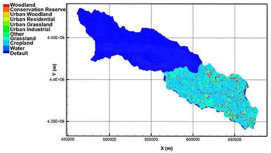
Though land use varied temporally throughout the post-1950 calibration period, land use in the HGS simulations did not. GIS-based land-use data are available only for 1990 and for 2000, and changes between these two datasets were minimal with respect to land-use characterization for the HGS model. As such, the 2000 dataset was used to characterize the model. As previously mentioned, characterization in the modeled region within Nebraska must be consistent with the RRCM. As no land-use data were incorporated into this model, a default property was used throughout the region. In addition, to minimize the effects of the transition between these two datasets, the land-use data within Kansas were implemented only within the surface sub-watershed that lies solely in Kansas (fig. 4).
Figure 4--Surface domain characterization in post-development HGS simulations.
Soils
Surface soil data from the Soil Survey Geographic database (SSURGO) were integrated into the landuse/land-cover classifications. The friction coefficient term in table 1 was estimated based on both landuse type and soil type. SSURGO data were used to determine the dominant soil for each land-use group, which was then used to better constrain the friction coefficient. This information does not change temporally as temporal datasets are not available.
Table 1--Surfaceflow parameters. Values from Julien (2002) and French (1994).
| Friction Coefficient (-) | Vegetative Cover (%) | |
|---|---|---|
| Woodland/ Riparian | 0.6 | 60 |
| Urban Residential | 0.012 | 0 |
| Urban Grassland | 0.2 | 10 |
| Urban Industrial | 0.012 | 0 |
| Other | 0.03 | 20 |
| Grassland | 0.22 | 10 |
| Cropland/Default | 0.2 | 30 |
| Water/ Streambed | 0.04 | 0 |
Boundary Conditions
For predevelopment conditions, the river inlet boundary was taken from documented streamflow measurements near Hardy, Nebraska, pre-1950 (Hansen, 1997). For simulations representing 1950-1990, inflow boundary conditions at the HCL outlet are taken from the USBR website, converting monthly acre-feet data into m3/s. No data are available from 1950 through 1952, so 1953 data are used for those years. After 1990, the coupled HGS-OASIS framework allows the Harlan reservoir releases in HGS to be taken from OASIS simulations. The stream outlet, as with the remainder of the surface edges, is a critical depth boundary.
Linking with OASIS
Post-1990 simulations use the linked HGS-OASIS framework developed for this work. These simulations link HGS to OASIS on a monthly basis (the OASIS time step). Each month, OASIS passes HGS the water released from HCL, Lovewell Reservoir and Jamestown Wildlife Area. OASIS also passes HGS information regarding water rights, whether Minimum Desirable Streamflow (MDS) administration is in effect, and the water released to irrigation canals. At the same time, HGS passes the quantity of groundwater recharge/discharge along stream sections to OASIS.
Geology and Lithology
Subsurface characterization is limited to three material types: top soil, alluvium, and bedrock (fig. 5). This simplification was necessary because of time constraints and project objectives. Drillers' logs are available for more detailed subsurface characterization throughout most of the simulated region. However, the time necessary to digitize the data and derive a conceptual model for simulation is beyond the resources available for this work. In addition, the objective of this work is to evaluate several surface water management alternatives. While groundwater/surface water interaction plays an important role in water availability for groundwater right holders, and for supporting ecological functions, it does not significantly influence the management of surface water operations. Although this assumption was confirmed through a preliminary sensitivity analysis, the influence of groundwater/surface water interactions on water management will be evaluated throughout this work.
Figure 5--Subsurface geology in HGS simulation of LRRB.
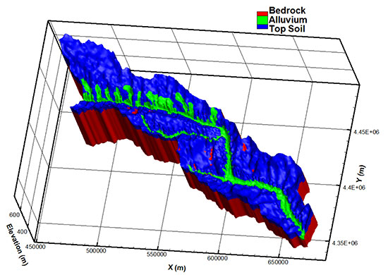
The bedrock layer was digitized from bedrock isolines in USGS OFR 1982-79 (Geohydrology of Principal Aquifers in the Republican River Basin, Kansas) and supplemented with drillers' logs from the following sources: Craig Haldeman Well Drilling & Pump Service, GeoCore Services Inc., Leroy Maruhn Well Drilling, Inc., Peterson Irrigation, Inc., Associated Environmental, Inc., Michael Peterson Irrigation, Inc., and Associated Drilling, Inc. The location of the alluvial aquifer along the Republican River in Kansas was taken from surface geology from a Kansas Data Access and Support Center (DASC) database that documents statewide alluvial aquifers based upon Quaternary alluvium and contiguous terrace deposits in statewide geology maps. The alluvial aquifer was extended to the bedrock interface. Within Nebraska, the location and depth of the bedrock and alluvium were made consistent with the RRCM. The remainder of the subsurface was classified as top soil. To ensure consistency with the RRCM, hydraulic conductivity, storage, and porosity values for both the alluvial material and the top soil were chosen to represent those used in the RRCM model and were found to be consistent with previous work in the LRRB (Sophocleous et al., 1997) (table 2). For bedrock, values were taken from the literature (see table 2). Van Genuchten parameters were taken from similar textures from the ROSETTA database (USDA, 2005).
Boundary Conditions
Both lateral and bottom subsurface boundary conditions were calibration parameters for the predevelopment simulations, as no data were available to characterize them. Initially, constant head boundaries were used along the lateral edges of the domain and a constant flux along the bottom. However, sensitivity analysis indicated that once the predevelopment simulations reached steady state, simulations with no-flow boundaries along the lateral edge achieved results consistent with simulations that used constant head boundaries. This is because comparatively little groundwater was flowing laterally through the boundaries to the alluvial aquifer as compared to that from above via precipitation, irrigation, and stream interaction. The calibrated bottom boundary flux was 8.5x10⁻⁹ m/s out of the domain.
Table 2--Subsurface parameters for HGS simulations.
| Bedrock | Alluvium | Top Soil | |||||
|---|---|---|---|---|---|---|---|
| Value | Source | Value | Source | Value | Source | ||
| Specific Storage | 0.000164 | Batu, 1998 | 0.000656 | Batu, 1998 | 0.000323 | Batu, 1998 | |
| Porosity | 0.25 | Freeze and Cherry, 1979 | 0.4 | RRCA Model | 0.37 | RRCA Model | |
| Hydraulic Conductivity |
0.00001 | Freeze and Cherry, 1979; Butler, 1998; Evans et al., 2001 |
0.00035 | RRCA Model | 0.0009 | RRCA Model | |
| Van Genuchten Parameters |
residual saturation |
0.053 | USDA, Evans et al., 2001 2005; | 0.063 | USDA, 2005 | 0.053 | USDA, 2005 |
| alpha | 2.5 | USDA, 2005; Evans et al., 2001 | 3.52 | USDA, 2005 | 7.5 | USDA, 2005 | |
Water Rights
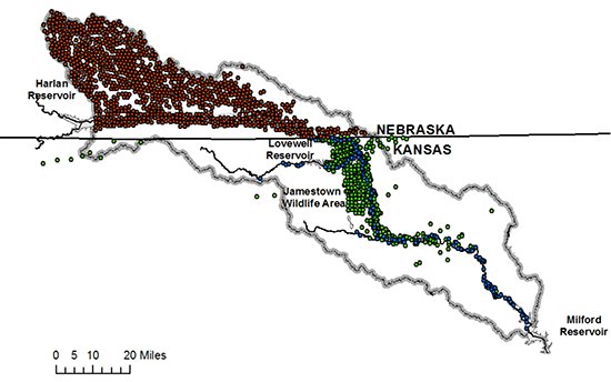
The LRRB contains both surface water and groundwater rights. Groundwater pumping records are readily available from the Kansas Department of Agriculture's Division of Water Resources (DWR) and are incorporated into this model (fig. 6). Well records were first mapped onto the HGS grid, combining records of any wells located on the same HGS node. Historical records of annual pumping volumes are then distributed over the growing season as guided by input from the irrigation district (1% in April, 3% in May, 14% in June, 50% in July, 30% in August and 2% in September).
There are two types of surface water diversions in the LRRB: those associated with an individual water right, similar to the groundwater rights, and those associated with an irrigation district. The surface water diversions associated with an individual water right are treated in the same manner as the groundwater rights, except that the place of extraction (river) is different from the application location (field). The irrigation districts have contracts with the USBR to release water directly from the reservoirs into irrigation canals for their use. The demand for irrigation districts is calculated by OASIS and is passed to HGS at each OASIS time step. Pumping wells within Nebraska are consistent with those in the RRCM (fig. 6).
Figure 6--Irrigation extraction points in LRRB model domain. Red dots indicate pumping wells in Nebraska, green dots indicate pumping wells in Kansas, and blue dots indicate surface water diversions in Kansas.
Irrigation Return Flow
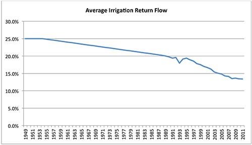
For groundwater rights, the return-flow of water from irrigation will be applied to the subsurface node below the root zone at the same areal location (in x, y) from which the water was extracted. Irrigation return flow was estimated based upon irrigation type within the basin (fig. 7), using the following returnflow estimates previously applied to studies in Kansas: 25% return flow for flood irrigation, 17% for center pivot and flood, 7% for center pivot with low energy precision application, 9% for center pivot with other sprinkler applications, and 4% for surface and subsurface drip irrigation (fig. 8; Wilson et al., 2008).
Figure 7--Reported irrigation types in the LRRB, Kansas, from 1949 to 2011.
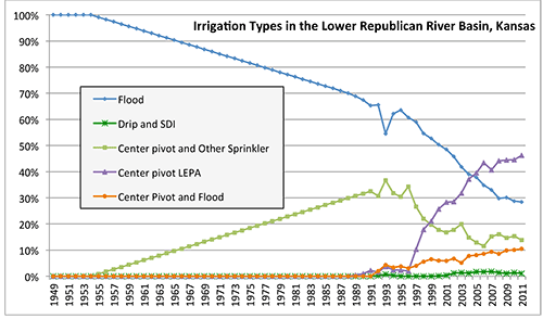
Figure 8--Average irrigation return flow in LRRB, Kansas, based upon irrigation type (fig. 7) and associated efficiency.
For surface water irrigation, the return-flow will be applied at the node closest to the discharge point for individual water rights. As irrigation districts have many end users and each demand cannot be attributed to anyone user or group of users, the water released for irrigation districts is applied evenly over a 20- node area within the district. Both irrigation pumping and application are applied as a constant rate throughout the irrigation season.
Climate parameters are applied to the domain as temporally averaged values over either seasonal (April to September--irrigating; October to March--non-irrigating) or monthly periods. Seasonal averages are applied to all simulations pre-1990, and monthly averages are used for post-1990 simulations.
Precipitation
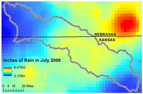
The PRISM (Parameter-elevation Regressions on Independent Slopes Model) Climate Data set is the source of historical precipitation data (http://www.prism.oregonstate.edu/).PRISM. which creates the USDA's official climatological dataset, is an analytical tool that combines point data, digital elevation models, and other spatial data to generate gridded estimates of climatic parameters, including precipitation and temperature. These data were converted to fluxes that are applied to the surface of the HGS domain as a raster file (one raster per forcing period), maintaining spatial variability in the study region (fig. 9).
Figure 9--Precipitation data set for July 2008 demonstrating spatial variability within the model domain.
Evapotranspiration
Average potential evapotranspiration (PET) was taken from Szilagyi (2001) for the Republican River Basin. PET is varied seasonally between growing and non-growing seasons. The total water pumped for irrigation that is not return-flow (as previously described) is subtracted from this value, giving the remaining PET after irrigation has been taken into account. This value is then divided by the surface area of the domain and is used as the PET demand for the simulation, which assumes this remaining demand will try to be met by incoming precipitation and soil-water storage.
Actual evapotranspiration is modeled as the combination of plant transpiration and surface and subsurface evaporation. Plant transpiration is estimated using the equation established by Kristensen and Jensen (1975). Evaporation is calculated on the vegetation cover (canopy evaporation) and from the surface and subsurface domains using the methods described in Therrien et al. (2007) and Li et al. (2008). The land use affects the evapotranspiration (ET) properties of the simulations. ET properties were taken from Kristensen and Jensen (1975), Canadell et al. (1996), Scurlock et al. (2001), and Therrien et al. (2007) (table 3).
Table 3--Evapotranspiration parameters used in the LRRB HGS simulations. Values from Kristensen and Jensen (1975), Canadell et at. (1996), Scurlock et al. (2001), and Therrien et al. (2007).
| Open Water |
Forest | Crop | Grass | Pavement | ||
|---|---|---|---|---|---|---|
| Evaporation Depth (m) | 0.1 | 2.0 | 2.0 | 1.5 | 0.1 | |
| Root Depth (m) | 0.0 | 3.0 | 2.1 | 2.1 | 0.0 | |
| Leaf Area Index (-) | 0.0 | 5.5 | 4.2 | 2.5 | 0.2 | |
| Transpiration Fitting Parameters |
C1 (-) | n/a | 0.3 | 0.3 | 0.3 | n/a |
| C2 (-) | n/a | 0.2 | 0.15 | 0.2 | n/a | |
| C3 (-) | n/a | 0.000003 | 1.0 | 0.000003 | n/a | |
| Transpiration Limiting Saturations |
Wilting Point (-) | n/a | 0.2 | 0.15 | 0.2 | n/a |
| Field Capacity (-) | n/a | 0.32 | 0.4 | 0.32 | n/a | |
| Oxic Limit (-) | n/a | 0.76 | 0.6 | 0.76 | n/a | |
| Anoxic Limit (-) | n/a | 0.90 | 0.8 | 0.9 | n/a | |
| Evaporation Limiting Saturations |
Minimum (-) | 0.1 | 0.2 | 0.15 | 0.1 | 0.1 |
| Maximum (-) | 0.5 | 0.42 | 0.4 | 0.5 | 0.5 | |
| Canopy Storage (m) | 0.0 | 0.07 | 0.05 | 0.04 | 0.05 | |
| Initial Interception Storage (m) | 0.0 | 0.07 | 0.05 | 0.04 | 0.05 | |
The OASIS model of the Lower Republican River Basin begins at the HCL in Nebraska and extends downstream to Clay Center, Kansas. The model includes Lovewell Reservoir on White Rock Creek and Jamestown Wildlife Area as well as all of the irrigation districts located between HCL and Lovewell Reservoir. Figure 10 shows a schematic of the LRRB model. The OASIS model routes surface water through the river and canal systems within the LRRB following the operation procedures for each of the reservoirs and demand patterns of the irrigation districts. The OASIS model of the LRRB was developed at the Kansas Water Office (KWO) and will be described in a future KWO report.
Figure 10--Schematic of LRRB model developed in OASIS.
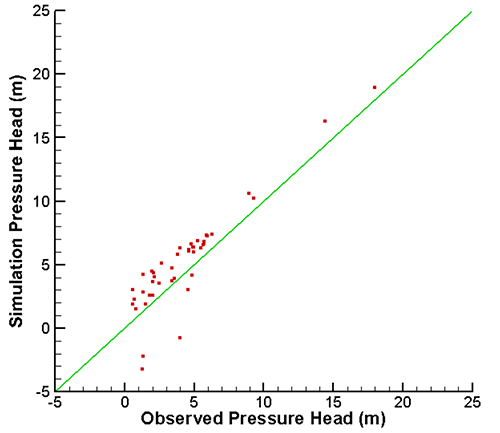
Initial conditions for the "spin up" simulations were fully saturated in the subsurface and 10-4 m of water on the entire surface. The simulation was run until the surface and variably saturated subsurface conditions reached a near-steady-state condition that represented pre-1950 (predevelopment) hydrology. The results from the predevelopment steady-state simulation were calibrated using available pre-1950 water-level data. Data from 52 wells were available for this period. Where multiple measurements took place at the same well, the values were averaged (KGS Wizard database; http://www.kgs.ku.edu/Magellan/WaterLevels/index.html). The surface flow conditions were calibrated using a single historic gage reported by the USGS (Clay Center) for 1952-1957. The parameter that was varied during calibration was the bottom boundary flux. Figure 11 provides calibrated pressure head (subsurface) values, which reasonably represented measured heads. The HGS model simulates a streamflow rate of 32 m3/s, which is reasonable compared to the average observed flow of 40 m3/s for 1940-1950 (range of 12-64 m3/s). Given the temporal variability of both surface and subsurface water levels, the lack of temporal and spatial data for calibration, and the steady-state conditions of the model, the results in fig. 11 indicate that the model provides an adequate representation of the predevelopment flow conditions. The purpose of these results is to provide reasonable initial conditions for the transient historic and recent development simulations.
Figure 11--Predevelopment observed vs. simulated pressure heads for the LRRB HGS model.
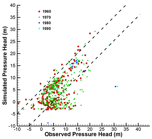
The transient calibration simulations were broken up into two phases. The first phase, simulating 1950-1990, was run with averaged seasonal (April through September; October through March) climatic, pumping, and irrigation parameters. Air temperature and precipitation values were taken from the PRISM Climate dataset. Average daily temperatures were calculated as the arithmetic average of the daily minimums and maximums. Groundwater pumping volumes for irrigation within Kansas were taken from reported water use, as archived by the KGS. Within Nebraska, groundwater pumping volumes were consistent with those used in the RRCM. As there are no reliable surface water diversion estimates for 1950-1990, surface water diversions were omitted until 1990-2010 transient simulations. Results from the 1950-1990 transient simulation were calibrated against groundwater levels at the start of each decade (fig. 12). The parameters varied during calibration were limited to those associated with evapotranspiration. As surface water diversions and surface water operations were not integrated into these simulations, the surface water levels were not used for calibration for this simulation, but they were used in the 1990-2010 simulation when OASIS was linked to HGS. Again, given the temporal variation of groundwater levels and the smoothing of climatic and irrigation forcings, the simulated groundwater pressure heads reasonably represent the observed values.
Figure 12--Simulated vs. observed pressure head for the 1950-1990 calibration period.
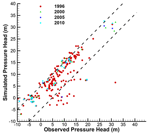
The second phase simulates 1990-2010. This phase was run with monthly climatic, pumping, and irrigation parameters using the same data sources used in the first phase of transient calibration. However, for this phase, surface water diversions were also included, derived from water-use reports collected by the DWR and archived by the KGS. In addition, HGS was linked to the surface water operations model of the LRRB to account for reservoir operations and releases to irrigation districts. Results from the 1990-2010 transient simulation were compared to groundwater levels for 1996, 2000, 2005, and 2010 (fig. 13); no further calibration of HGS data inputs were conducted for the 1990-2010 period; this was used as the HGS verification period. The surface runoff component in OASIS was varied during this period to calibrate the linked model. Surface water levels at HCL, Lovewell Reservoir, and USGS gage stations along the Republican River from the OASIS framework were compared to observed data. Both the surface water levels and groundwater levels are representative of observed values. Groundwater levels are slightly over-estimated, which a preliminary sensitivity analysis indicates may be due to irrigation return-flow assumptions. Given the project deadlines and the long run times of these simulations, a complete sensitivity and uncertainty analysis could not be completed. This will be the focus of future work.
Figure 13--Simulated vs. observed pressure head for the 1990-2010 calibration period.
As an integrated surface/subsurface hydrologic model, HGS can provide information about the surface, the subsurface, and the interactions between them. Due to the dependence of the surface water system on structural and operational components, HGS is not used for surface water analysis in this project; the results from OASIS provide that information. HGS is used to analyze the groundwater conditions and the exchange of water between the surface and subsurface. The results presented here focus on the 1990- 2010 calibration and verification period.
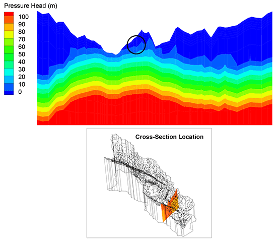
Groundwater conditions vary spatially and temporally throughout the LRRB in response to variations in groundwater pumping, irrigation application, precipitation, and reservoir releases. Figure 14 demonstrates the spatial variability of total hydraulic head across the domain; most of the variability in total hydraulic head is due to variations in topography. As shown in fig. 15, the pressure head varies spatially due to water levels in the stream, as driven by reservoir releases and precipitation. These changes also vary temporally in the streambed, with higher pressure heads when large reservoir releases or precipitation events occur, reflecting higher water levels in the stream. Changes in the pressure head are also visible at depth in the vicinity of the stream and groundwater pumping wells, as shown in a cross section through the domain (fig. 16). These changes also vary temporally as a result of the seasonal operations of irrigation pumping wells.
Figure 14--Sample of total hydraulic head results (January 2005).
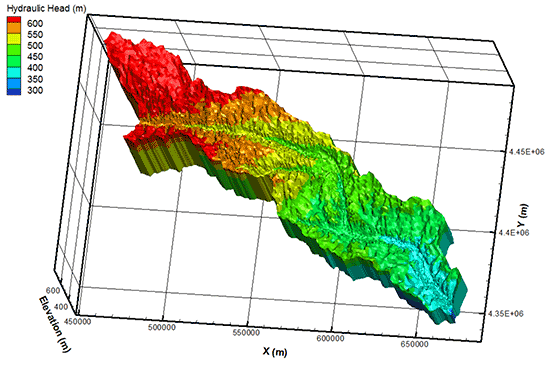
Figure 15--Sample of pressure head results (January 2005).
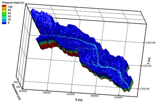
Figure 16--Cross section of domain (location shown in inset) illustrating pressure head variations with depth (April 2006). Black circle indicates an example of decreased head due to groundwater pumping.
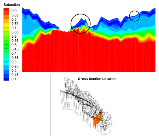
The spatial nature of both precipitation and irrigation application cause their effects to be muted in head response compared to the focused nature of stream levels and groundwater pumping. As a result, the effects of precipitation and irrigation application are most visible in saturation results (fig. 17). Increases in saturation at the surface occur during the irrigation season and during times of increased precipitation.
Figure 17--Cross section of domain (location shown in inset) illustrating saturation variations with depth (April 2006). An increase in saturation is evident at the surface (examples circled) demonstrating the movement of precipitation and irrigation flow through the vadose zone.
Groundwater/surface water (gw/sw) exchange fluxes are dependent on surface and shallow subsurface conditions. As such, gw/sw exchange fluxes have greater variability both spatially and temporally compared to the groundwater conditions, particularly in the streambed (fig. 18). Within the streambed, spatial variability is most dependent on changes in topography, including the locations of pools, riffles, and other streambed features. These features cause drastic changes in gw/sw exchange fluxes (from gaining to losing) along the streambed (fig. 18). In other cases, variations in hydraulic conductivity also cause these spatial variations (e.g., Schornberg et al., 2010, and Kalbus et al., 2009). However, the LRRB model maintains a homogeneous alluvium. Temporal variations in gw/sw interactions within the streambed are caused primarily by irrigation demands, groundwater pumping in the alluvial aquifer, and reservoir releases. During irrigation season, the losing portions of the stream became greater and some regions switched from gaining to losing. This is due to groundwater pumping in the alluvium drawing water from the stream. In addition, during the irrigation season, there are often short-term increases in the stream levels as water is released from reservoirs for irrigation districts. These releases cause temporary increases in the surface water heads, causing stronger gradients into the subsurface.
Figure 18--Exchange flux (L/m2d) results (June 2006). Negative values indicate water recharging the subsurface; positive values discharge to the surface.
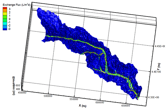
The only variations in groundwater/surface water exchange in the upland regions are due to changes in precipitation and evapotranspiration. Water is always infiltrating into the subsurface in these regions. That infiltration, however, is quite homogeneous throughout the upland areas (fig. 18).
This linked OASIS/HGS model was developed and calibrated to evaluate several alternatives for watermanagement strategies in the LRRB, under current and projected future climates. This work is ongoing and will be a part of a future OFR.
Kansas is evaluating one structural and one operational water management alternative through this study. The structural change is the expansion of Lovewell Reservoir in combination with the winterization and automation of the Courtland Canal system. Three expansion volumes will be evaluated: 16,000 AF, 25,000 AF, and 35,000 AF. Winterization of the canals includes the addition of bubbles systems at each radial gate of check structures and the canal headworks at the diversion dam. Automation of the radial gates at the check structures and headworks of the diversion dam will allow individual radial gate control.
The operational alternative that Kansas is evaluating is the use of the Jamestown Wildlife Area for offseason storage of surplus water from Lovewell Reservoir or Courtland Canal to allow the state to better meet the needs of wildlife habitat and to alter the release of water in response to MDS and other water-use requirements downstream.
The climate projections for this study are obtained from an archive of bias-corrected and spatially disaggregated (BCSD) climate projections developed by USBR in partnership with the USGS, U.S. Army Corps of Engineers, Lawrence Livermore National Laboratory, Santa Clara University, Climate Central, and Scripps Institution of Oceanography. A subset of the BCSD projections will be selected to represent the full ensemble of projected changes in temperature and precipitation. Three projections will be selected: one projection to represent the central tendency of the ensemble and two projections to represent the range of the ensemble. One will represent a hotter and drier climate, and one a less hot and wetter climate. These simulations will be run in conjunction with results from future climate and watermanagement alternative scenarios simulated by Nebraska.
Batu, V., 1998, Aquifer hydraulics: A comprehensive guide to hydrogeologic data analysis: New York, John Wiley.
Breuer, L., Eckhardt, K., and Frede, H.-G., 2003, Plant parameter values for models in temperate climates: Ecological Modelling, v. 169, p. 237-293.
Butler, Jr., J. J., 1998, Type-curve analysis of July 1997 pumping tests in the Dakota well field of the City of Hays, Ellis County, Kansas: Kansas Geological Survey, Open-File Report 98-15a, 55 p. [available online]
Canadell, J., Jackson, R. B., Ehleringer, J. R., Mooney, H. A., Sala, O. E., and Schulze, E.-D., 1996, Maximum rooting depth of vegetation types at the global scale: Oecologia, v. 108, p. 583-595.
Dunlap, L. E., 1982, Geohydrology of principal aquifers in the Republican River basin, Kansas: U.S. Geological Survey Open-File Report 82-19.
Evans, D. D., Nicholson, T. J., and Ramussen, T. C., eds., 2001, Flow and transport through unsaturated fractured rock: American Geophysical Union, Geophysical Monograph Series, v. 42, 196 p.
Freeze, R. A., and Cherry, J. A., 1979, Groundwater: London, Prentice-Hall International, 6,044 p.
French, R. H., 1994, Open Channel Hydraulics: New York, McGraw-Hill.
Hansen, C. V., 1997, Major components of flow in the Republican River during drought conditions from near Hardy, Nebraska, to Concordia, Kansas: U.S. Geological Survey, Fact Sheet 234-96.
Hollinger, D. Y., Ollinger, S. V., Richardson, A. D., Meyers, T. P., Dail, D. B., Martin, M. E., Scott, N. A., Arkebauer, T. J., Baldocchi, D. D., Clark, K., Curtis, P. S., Davis, K., Desai, A., Dragoni, D., Goulden, M. L., Gu, L., Katul, G. G., Pallardy, S., Paw U, K. T., Schmid, H., Suyker, A. E., and Verma, S. B., 2010, Albedo estimates for land surface models and support for a new paradigm based on foliage nitrogen concentration: Global Change Biology, v. 16, no. 2, p. 696-710.
Hydrologics, 2009, OASIS with OCL, Model Version 3.10.8, GUI version 4.6.16., 339 p.
Jensen, M., and Haise, H., 1963, Estimating evapotranspiration from solar radiation: Journal of Irrigation and Drainage Division, ASCE, v. 89, no. 1, p. 15-41.
Julien, P. Y., 2002, River Mechanics: Cambridge, UK, Cambridge Press.
Kalbus, E., Schmidt, C., Molson, J. W., Reinstorf, F., and Schirmer, M., 2009, Influence of aquifer and streambed heterogeneity on the distribution of groundwater discharge: Hydrology and Earth System Sciences, v. 13, p. 69-77.
Kristensen, K. J., and Jensen, S. E., 1975, A model for estimating actual evapotranspiration from potential transpiration: Nordic Hydrology, v. 6, p. 170-188.
Li, Q., Unger, A. J. A, Sudicky, E. A., Kassenaar, K., Wexler, W. J., and Shikaze, S., 2008, Simulating the multi-seasonal response of a large-scale watershed with a 3D physically-based hydrologic model: Journal of Hydrology, v. 357, p. 317-336.
Nebraska and Kansas, 2005. Lower Republican River Basin Appraisal Report. http://www.usbr.gov/gp/nkao/fext050121final.pdf
Panday, S., and Huyakorn, P. S., 2004, A fully coupled physically-based spatially-distributed model for evaluating surface/subsurface flow: Advances in Water Resources, v. 27, p. 361-382, doi:10.1016/j.advwatres.2004.02.016
Perkins, S. P., and Sophocleous, M. A., 1997, Lower Republican stream-aquifer project, final report; volume 2, development and documentation of a combined watershed and stream-aquifer modeling program: Kansas Geological Survey, Open-File Report 97-9, 164 p.
Republican River Compact Administration, 2003, Republican River Compact Administration Ground Water Model, June 30, 2003. http://www.republicanrivercompact.org/v12p/RRCAModelDocumentation.pdf
Schornberg, C., Schmidt, C., Kalbus, E., and Fleckenstein, J. H., 2010, Simulating the effects of geologic heterogeneity and transient boundary conditions on streambed temperatures--Implications for temperature-based water flux calculations: Advances in Water Resources, doi:10.1016/j.advwatres.2010.04.007.
Scurlock, J. M. O., Asner, G. P., and Gower, S. T., 2001, Worldwide Historical Estimates of Leaf Area Index, 1932-2000: Oak Ridge National Laboratory, U.S. Department of Energy (DE-AC05-00OR22725). [available online]
Sophocleous, M. A., Perkins, S. P., Moustakas, S., and Kaushal, R. S., 1995, Republican River stream/aquifer study; model development and applications, 1995 year-end progress report to KWO: Kansas Geological Survey, Open File Report 95-53, 106 p.
Sophocleous, M. S., Perkins, S. P., Stadnyk, N. G., and Kaushal, R. S., 1997, Lower Republican Stream-Aquifer Project: Final Report: Kansas Geological Survey, Open-File Report 97-8, 131 p.
Szilagyi, J., 2001, Identifying the cause of declining flows in the Republican River: Journal of Water Resources Planning and Management, v. 127, p. 244-253.
Therrien, R., McLaren, R. G., Sudicky, E. A., and Panday, S. M., 2007, HydroGeoSphere: a three-dimensional numerical model describing fully-integrated subsurface and surface flow and solute transport: Groundwater Simulations Group, University of Waterloo, Waterloo, Ontario, Canada.
U.S. Department of Agriculture Agricultural Research Service, 2005, ROSETTA class average hydraulic parameters: http://www.ars.usda/gov/Services/docs.htm?docid8955. Accessed December 2012.
Vazquez, R. F., and Feyen, J., 2003, Effect of potential evapotranspiration estimates on effective parameters and performance of the MIKE SHE-code applied to a medium-size catchment: Journal of Hydrology, v. 270, p. 309-327.
Wilson, B. B., Liu, G., Whittemore, D., and Butler, J. J., 2008, Smoky Hill River Valley Ground-water Model: Kansas Geological Survey, Open-File Report 2008-20, 103 p. [available online]
Kansas Geological Survey, Geohydrology
Placed online Feb. 18, 2015
Comments to webadmin@kgs.ku.edu
The URL for this page is http://www.kgs.ku.edu/Hydro/Publications/2015/OFR15_1/index.html