Kansas Geological Survey, Open-file Report 98-15A
KGS Open File Report 98-15A
May 1998
The complete report is available as an Adobe Acrobat PDF file (415 kB).
Two multi-day pumping tests were performed by the Kansas Geological Survey in the Dakota well field of the city of Hays in Ellis County, Kansas in July of 1997. The major objective of these tests was to obtain information about the hydraulic and geochemical responses of the well field to extended periods of pumping. Type curve analyses were performed on the drawdown data from the observation well closest to each pumping well. The purpose of these analyses was to obtain parameter estimates for input to a numerical model of the well field. The transmissivity (T) and storativity (S) of the Dakota sands estimated for the vicinity of well D6 were 584 ft2/d and 6.95 X 10⁻⁵, respectively. The T and S of the Dakota sands estimated for the vicinity of well D-1 were 859 ft2/d and 9.49 X 10⁻⁵, respectively. These parameter estimates are in good agreement with those obtained from pumping tests performed at the same wells in 1992. Plots of drawdown versus time from both tests clearly show that the Dakota sands are of limited width in the well field and are bounded by units of relatively low permeability. Both drawdown and recovery plots indicate that there is a significant component of recharge into the Dakota sands during the course of these tests. Although the source of this recharge cannot be determined on the basis of these analyses, leakage from adjacent low-permeability units is probably the most significant recharge mechanism.
Two multi-day pumping tests were performed by the Kansas Geological Survey (KGS) in the Dakota well field of the city of Hays in Ellis County, Kansas in July of 1997. This work was done as part of an extension of the Dakota Aquifer Program, a multi-year research effort of the KGS directed at developing an understanding of the hydrologic, water-quality, and water-resources-management ramifications of increased utilization of the Dakota aquifer in central and western Kansas (Macfarlane et al., 1990). This extension of the Dakota Aquifer Program was funded by the city of Hays for the specific purpose of evaluating the long-term effect of water-resources development on the Dakota aquifer in the vicinity of the city's Dakota well field. P. Allen Macfarlane of the Geohydrology Section of the KGS served as the principal investigator for this project.
The two pumping tests that are the subject of this report were performed to gather more information about the hydraulic and geochemical responses of the well field to extended periods of pumping. This report describes the results of type curve analyses of the drawdown data collected at the observation well closest to each pumping well. The parameter estimates obtained from these analyses served as input to a numerical model used to simulate the well field response to the pumping stresses. That simulation investigation is described in a separate report.
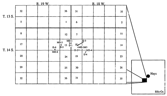
The location of the well field is in Ellis County, just south of the city of Hays, Kansas. Figure 1 shows the position of the well field relative to the city of Hays, and the distribution of pumping and monitoring wells within the well field. During July of 1997, multi-day pumping tests were performed at wells D-6 and D-1. Prior, during, and after these tests, depth to water measurements were obtained at all of the wells shown on Figure 1 using a Solinst electric tape. At monitoring wells MD-6, MD-1, and MD-2&3, these manually collected data were supplemented by measurements obtained with pressure transducers (In-Situ PXD-261 series 0-10 and 0-20 psig transducers) connected to data loggers (Campbell Scientific 21X and CR500 loggers). Use of the pressure transducers enabled changes in water levels at these wells to be monitored at a much higher frequency than would be possible by manual means. During a pumping test, changes in water level at an observation well are primarily a function of the portions of the aquifer lying radially outward from the observation well (Butler, 1990). Thus, observation wells close to a pumping well can be the source of valuable information about the hydraulic properties of an aquifer. Transducers were placed in wells MD-6 and MD-1 so that a very extensive series of drawdown data could be obtained from the monitoring well closest to the pumping well in each test. The analysis of these drawdown data using conventional type-curve methods is the subject of this report. Note that since water levels were over 100 ft above the top of the Dakota sands in all of the wells during these two pumping tests, the Dakota sands are classified as a confined aquifer for the purposes of this report. Since changes in atmospheric pressure can induce changes in water level within a confined aquifer (Kruseman and de Ridder, 1990), barometric pressure was also monitored during the course of these tests. In this report, barometric pressure data obtained with a pressure transducer (Setra Model 270 800-1100 millibar) located at well MD-1 will be briefly discussed. At both D-6 and D-1, the pumping rate was measured using in-line flowmeters previously installed by the city of Hays. No field checks on the flowmeter readings could be obtained during these tests. A complete discussion of the pumping tests, along with details concerning the hydrogeology of the well field and its vicinity, can be found in a separate report.
Figure 1--Location map for the Dakota well field of the city of Hays (pumping wells labelled with prefix "D" and monitoring wells labelled with prefix "MD")
The drawdown and recovery measurements were analyzed by comparing the data to theoretical models that were thought to closely resemble the test configuration. In this work, two theoretical models of pumping tests in confined aquifers were employed: 1) the infinite aquifer model of Theis (Kruseman and de Ridder, 1990), and 2) the linear strip model of Butler and Liu (1991). The infinite aquifer model of Theis was considered a logical model for analysis of the early portions of the pumping tests, for the period prior to the time at which the lateral boundaries of the Dakota sands began to significantly affect the drawdown data. The linear strip model of Butler and Liu was derived for the purpose of analyzing well tests in conditions where the aquifer consists of a permeable strip (channel) embedded in a matrix of lower permeability (e.g. the Dakota sands in the vicinity of the Hays well field), so it was considered a logical model for analysis of the portions of the pumping tests after the lateral boundaries began to significantly affect the drawdown data. Analyses using the Theis model were performed with SUPRPUMP, an automated well-test analysis package developed at the Kansas Geological Survey (Bohling et al., 1990; Bohling and McElwee, 1992), while analyses performed with the strip model of Butler and Liu involved manual comparisons of data plots with plots of the theoretical drawdown.
The analysis of the drawdown and recovery data consisted of three phases. In the first phase, the drawdown data were analyzed with the infinite aquifer model of Theis. The objective of this analysis step was two-fold: 1) to obtain estimates of transmissivity and storativity that are unaffected by boundary influences; and 2) to define the time at which lateral boundaries began to affect the drawdown data. In phase two, the drawdown data were analyzed with the strip model of Butler and Liu. This analysis step had three objectives: 1) to estimate the distance from the pumping well to lateral boundaries with units of lower permeability; 2) to estimate the minimum contrast in transmissivity across the lateral boundaries; and 3) to check on the transmissivity and storativity estimates obtained with the Theis model. In phase three, the recovery (residual drawdown) data were analyzed with the Butler and Liu strip model using the format of the Theis recovery method (Kruseman and de Ridder, 1990). This analysis step had two objectives: 1) to check on the estimates obtained in the previous two steps; and 2) to assess the impact of recharge on the drawdown data. Note that the term recharge is used here in its most general sense to designate any mechanism that adds water to the Dakota well field. Thus, for example, recharge could be a product of leakage from adjacent low-permeability units or of lateral flow in the sands driven by previous pumping activities. In cases where the influence of recharge is not great, its presence can often be best recognized from plots in the format of the Theis recovery method.
In the following two sections, the results of this three-step analysis procedure are presented for the D-6 and D-1 pumping tests.
Well D-6 was pumped at an approximately constant rate of 77 gallons per minute (gpm) from July 7 to July 14, 1997. The total duration of the pumping period was 168.65 hours (607,151 secs). After the pump was cut off, water levels were allowed to recover for 95.68 hours (344,445 secs) prior to commencement of pumping at well D-1. Collection of recovery data continued until the pumping at D-1 began to affect water levels at MD-6. Since it took over six hours (21,948 secs) for that to occur, the total duration of the pumping and recovery period at well MD-6 was 270.43 hours (973,544 secs). A total of 10,431 transducer readings were acquired during this period. Figure 2 is a logarithm of time since pumping began versus drawdown plot that includes the entire pumping and recovery period used in the analysis at well MD-6. As shown by this plot, the pump in D-6 operated continuously for the entire pumping period of 168.65 hours. Table 1 provides well construction information for wells D-6 and MD-6.
Figure 2--Plot of the logarithm of time since pumping began versus drawdown for the D-6 pumping test (drawdown measured with transducer in well MD-6).
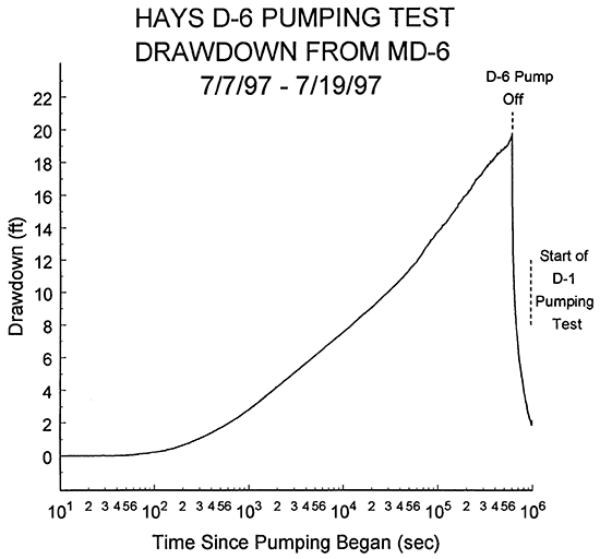
Table 1--Well construction information for wells D-6 and MD-6 in Dakota well field of the city of Hays.
| Well No.1 | Borehole Radius2 |
Casing Radius (ESR)3 |
Total Depth4 |
NSI4,5 | Sand Thickness6 |
|---|---|---|---|---|---|
| D-6 | 0.833 | 0.359 (0.833) |
545 | 484-544 | 63 |
| MD-6 | 0.333 | 0.081 (0.333) |
548 | 486-502 512-547 |
30 |
| 1 - distance between wells is 261 ft. 2 - units for information in this and remaining columns are ft. 3 - ESR--effective screen radius 4 - depths are from land surface 5 - NSI--nominal screened interval 6 - estimates provided by P. Allen Macfarlane |
|||||
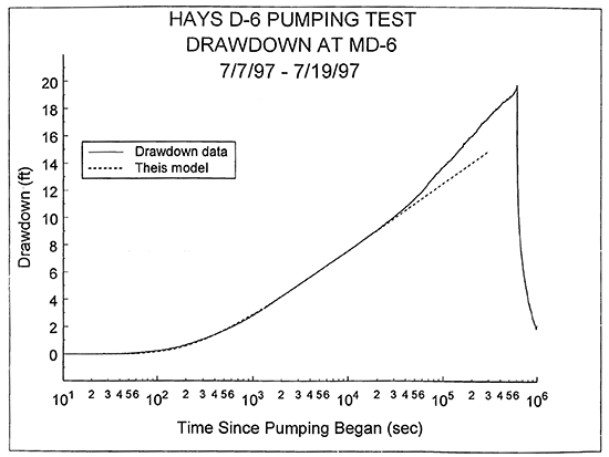
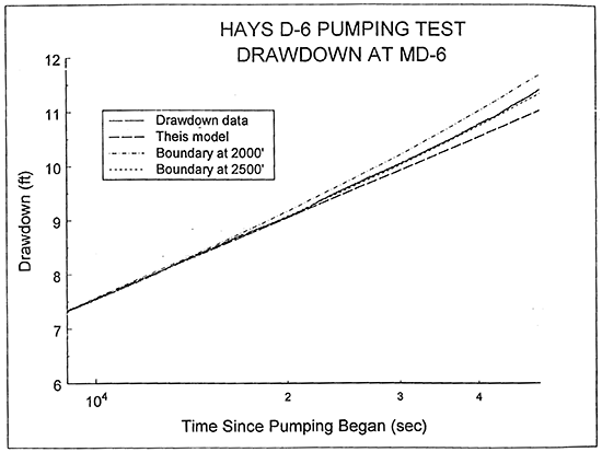
The first phase of the analysis process was to analyze the drawdown data with the Theis model. The concave-upward curvature of the drawdown plot of Figure 2 is an indication that lateral boundaries are affecting drawdown during the pumping period. Thus, the strategy used with the Theis model was to initially analyze very early time data and then systematically extend the upper time limit of the drawdown data used in the analysis until boundary effects began to impact the results. The parameter estimates obtained from the analysis immediately prior to the appearance of boundary effects were considered the most reasonable estimates of transmissivity and storativity for the Dakota sands in the vicinity of wells D-6 and MD-6. Figure 3 displays the final Theis model resulting from this procedure. Note that the drawdown data begin to deviate from the Theis model at approximately 20,000 seconds after the start of pumping. The transmissivity and storativity estimates obtained from the analysis were 544 ft2/day and 6. 48 X 10-5, respectively. These values were checked by performing a Cooper-Jacob analysis (Kruseman and de Ridder, 1990) of the straight-line segment of the drawdown plot of Figure 3 (2,000-20,000 seconds). The transmissivity and storativity values obtained in this manner were within 3% and 10%, respectively, of the values calculated with the Theis model.
Figure 3--Logarithm of time since pumping began versus drawdown plot and the best-fit Theis type curve for the D-6 pumping test (drawdown measured with transducer in well MD-6).
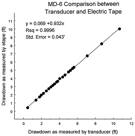
The estimates given in the previous paragraph were obtained using only the data from the pressure transducer in well MD-6. Butler (1997) emphasizes the importance of checking transducer operation in the field. For this project, transducer operation was checked by comparing readings from the transducer with electric tape measurements taken at the same time. Figure 4 is a plot of drawdown as measured by the transducer in well MD-6 versus drawdown as measured in MD-6 with an electric tape. The slope of 0.932 for the best-fit line indicates that the calibration parameters for the transducer were producing a systematic over-prediction of drawdown. This systematic over-prediction led to an underprediction of both transmissivity and storativity. Thus, the transmissivity and storativity estimates had to be corrected for the small errors in the calibration parameters. This correction was done by multiplying the parameter estimates determined for the Theis model by the inverse of 0.932 (1.073). The resulting transmissivity and storativity estimates were 584 ft2/day and 6.95 X 10⁻⁵, respectively. Note that these values are within 12% and 4%, respectively, of estimates obtained from an analysis of a 1992 pumping test performed at well D-6 using drawdown from well MD-6 (P. Allen Macfarlane, personal communication).
Figure 4--Calibration plot for transducer in well MD-6 (eqn. for best-fit line, and R2 and standard error of regression given in upper left-hand corner; electric tape measurements collected by P. Allen Macfarlane).
The second phase in the analysis process was to compare the drawdown data to theoretical plots produced by the Butler and Liu model. The first step of this phase was to estimate the position of the closest lateral boundary. Figure 5 is a plot of the logarithm of time since pumping began versus drawdown for the time interval during which a lateral boundary first began to affect the drawdown data. The measured drawdown is plotted along with theoretical curves for drawdown in an infinite aquifer (Theis model) and for aquifers with single linear boundaries at different distances from the pumping well. In this case, the theoretical drawdown for a linear boundary at 2500 ft from the pumping well appears to most closely match the measured data. This theoretical drawdown was computed assuming that well MD-6 lies between the pumping well and the boundary on a line that is perpendicular to the boundary, and that transmissivity decreased by two orders of magnitude across the boundary (storativity did not change). This transmissivity contrast was the minimum contrast that could be used to reproduce the drawdown data. The deviation of the plot of the measured drawdown from the theoretical drawdown curve seen at the upper end of the time range plotted on Figure 5 is probably an indication that the contrast is larger than two orders of magnitude. Note that the exact distance from the boundary to the pumping well cannot be determined on the basis of this analysis, although bounding values can be calculated using image-well theory (Kruseman and de Ridder, 1990). The distance of 2500 ft used here is actually the maximum possible distance to the boundary. The minimum distance to the boundary would occur for the case of a boundary perpendicular to the line connecting D-6 and MD-6, but lying on the opposite side of D-6 from MD-6. In that case, the boundary would lie at a distance of approximately 2239 ft from the pumping well. If the boundary is parallel to the line connecting wells D-6 and MD-6, the distance to the boundary is approximately 2370 ft. Thus, the boundary is somewhere between 2239-2500 ft from the pumping well, the exact distance depending on the location of the boundary relative to the position of the wells. For the purposes of the plots and discussions of this report, the maximum distance of 2500 ft is used in all cases.
Figure 5--Plot of the logarithm of time since pumping began versus drawdown for the D-6 pumping test with the best-fit Theis type curve and strip-model type curves for a single linear boundary (drawdown measured with transducer in MD-6; plot for interval of time during which first lateral boundary began to affect drawdown).
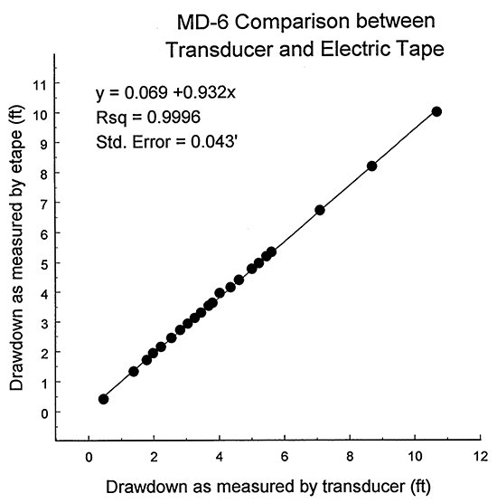
Figure 6 is a plot of the logarithm of time since pumping began versus drawdown for the remainder of the pumping test after the interval depicted in Figure 5. Theoretical curves are plotted for different transmissivity contrasts across a single linear boundary along with the barometric pressure record from the transducer (electronic barometer) at MD-1. This plot indicates that the transmissivity contrast across the boundary is greater than two orders of magnitude. There are two important features to note on this figure: 1) the increase in drawdown over that seen with a single linear boundary for times between 60,000-80,000 seconds; and 2) the decline in the rate of drawdown, relative to the single linear boundary case, for times greater than 100,000 seconds. Each of these features is discussed in the following paragraphs.
Figure 6--Plot of the logarithm of time since pumping began versus drawdown for the D-6 pumping test with the strip-model type curves for a single linear boundary and the barometric pressure record (drawdown measured with transducer in MD-6; barometric pressure measured with transducer at MD-1; type curves for different order-of-magnitude transmissivity contrasts across boundary).
Several mechanisms could be invoked to explain the increase in drawdown between 60,000-80,000 seconds. These include 1) a very large contrast in transmissivity across the boundary; 2) the start up of a nearby pumping well; 3) an increase in atmospheric pressure; 4) a second lateral boundary; 5) an increase in the rate of pumping at D-6; and 6) undulations in the position of a single boundary. Figure 6 depicts theoretical curves for transmissivity contrasts of up to four orders of magnitude. Curves for greater contrasts would lie extremely close to the four-order contrast curve over the time range displayed in Figure 6. Thus, the increase in drawdown is not due to a very large contrast in transmissivity across the boundary. Similarly, outside of the other pumping wells of the city of Hays (all of which were off), there appear to be no wells in the vicinity of D-6 capable of pumping at the rate necessary to produce the observed deviation. The barometer record on Figure 6 indicates that barometric pressure variations have little impact on drawdown at MD-6 during this time period. The major impact of barometric pressure appears to have been on the last day of the test where a significant increase in barometric pressure near 500,000 seconds approximately coincides with an increase in the rate of drawdown. Note that barometric pressure variations had such little impact on drawdown during the D-6 and D-1 pumping tests that barometric-pressure-induced fluctuations were not removed from the drawdown data for either test. Thus, in both tests, the late-time drawdown display small-amplitude oscillations (e.g., Figure 6) that are a product of variations in barometric pressure. These oscillations, however, had no impact on the analyses performed for this report.
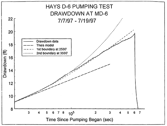
The increase in drawdown is most probably the product of an additional lateral boundary impacting the drawdown data. Figure 7 is a plot of the logarithm of time since pumping began versus drawdown that includes the theoretical curve for drawdown in an aquifer with two parallel boundaries on either side of D-6 at distances of 2500 and 3500 ft from the well. Although recharge begins to impact drawdown relatively shortly after the deviation from the single boundary case, the drawdown data and the theoretical curve for the case of a second linear boundary are in good agreement for close to 30,000 seconds after divergence from the single boundary curve. Thus, this analysis indicates that the Dakota sands are approximately 6,000 ft in width in the vicinity of D-6, a finding that is in reasonable agreement with maps of the thickness of the Dakota sands in the well field. Note that the 3500 ft distance to the second boundary is the minimum distance to that boundary. The maximum distance to the second boundary (3761 ft) would correspond to the minimum distance to the first boundary (2239 ft). Although other possibilities for the divergence are a short-term increase in pumping rate and undulations along a single boundary, neither of these appear as probable as a second boundary.
Figure 7--Plot of the logarithm of time since pumping began versus drawdown for the D-6 pumping test with the best-fit Theis type curve and strip-model type curves for one and two linear boundaries (drawdown measured with transducer in MD-6; two linear boundaries are assumed to be parallel).
Figures 6 and 7 clearly show that the rate of drawdown begins to decrease, relative to the theoretical models, at times greater than 100,000 seconds. Although this decrease could have been produced by a long-term decrease in pumping rate, pumping rate measurements obtained over this period do not show such a decrease. Thus, the most likely cause is recharge into the Dakota sands in the vicinity of well D-6. There are several potential sources of this recharge. It is possible that the decrease in the rate of drawdown is produced by a significant increase in the width, thickness, and permeability of the sand deposits with distance from the pumping well. This increase would result in significantly more lateral flow into the well field in the vicinity of D-6 than would be predicted from the theoretical models used in this analysis. It is doubtful, however, if this mechanism could provide sufficient water to produce the observed decrease in the rate of drawdown. Perhaps a more reasonable explanation is leakage from the low-permeability units that surround the Dakota sands. Given the large surface area of the contact between the Dakota sands and the surrounding units, the necessary rate of leakage per unit area would be very small. There is also the likely possibility that a portion of the recharge is a product of recovery from previous pumping in the Dakota well field. Extended monitoring of water levels in MD-6 after the D-1 pumping test revealed that the well field was far from static conditions at the start of the D-6 test. Transducer readings at MD-6 over the 922 minutes immediately prior to the start of the D-6 pumping test recorded an increase in water level of at least 0.15 ft. If that rate is projected over the entire period of the test, over 1.6 ft of increase would occur. Thus, a component of the recharge was undoubtedly a product of recovery from previous pumping activities. Although it is impossible to precisely define the cause of the decline in the rate of drawdown from an analysis of drawdown at MD-6, leakage from adjacent low-permeability units and recovery from previous pumping activities are probably the two most significant mechanisms.
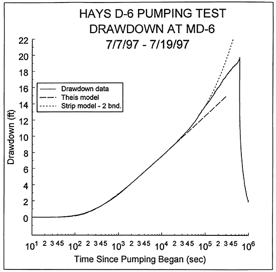
Figure 8 displays the results of the second phase of the analysis of the MD-6 data. The relatively close match between the measured drawdown and the strip model of Butler and Liu is a further demonstration of the validity of the transmissivity and storativity estimates obtained in the first phase of the analysis.
Figure 8--Plot of the logarithm of time since pumping began versus drawdown for the D-6 pumping test with the best-fit Theis type curve and strip-model type curve for two linear boundaries (drawdown measured with transducer in MD-6; two linear boundaries are assumed to be parallel).
The final phase of the analysis of the MD-6 data was an examination of the recovery data. Figure 9 is a plot of the data in the format of the Theis recovery method (logarithm of the ratio of the total time since pumping began over the time since pump turned off versus residual drawdown). The large dashed line depicts the residual drawdown for the strip model using a transmissivity contrast of three orders of magnitude, and assuming that pumping at D-1 does not affect the recovery data. As would be expected from theory, the plot converges on a residual drawdown of zero as the time ratio goes to one. The measured residual drawdown, however, do not display this same convergence. Even though pumping at well D-1 begins to impact the residual drawdown prior to complete recovery , it is clear that the plot is not converging on a residual drawdown of zero as the time ratio goes to one. Instead, it appears that a negative residual drawdown would be obtained at a time ratio of one. As shown by Streltsova (1988), recovery data that display this form are being affected by recharge. Note that the difference between the residual drawdown data and the strip model at large time ratios (i.e. immediately after cessation of pump age at D-6) is a product of the difference shown on Figure 8 between the measured and theoretical drawdown at the time the pump was cut off.
Figure 9--Plot of the log of the ratio of the total time since pumping began over the time since pump was cut off versus the residual drawdown for the D-6 pumping test with three strip-model type curves (residual drawdown measured with transducer in MD-6i modifications to the strip model described in text).
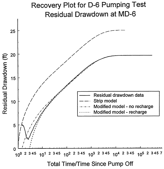
The effect of recharge on the recovery data can be readily demonstrated through two modifications to the strip model. The first modification consists of subtracting 5.31 ft from the drawdown computed using the strip model, which makes the measured and computed recovery plots coincide at large time ratios. The curve entitled "Modified model - no recharge" depicts the theoretical drawdown for this case. As shown on Figure 9, the assumption of no recharge produces a significant divergence between the theoretical model and measured residual drawdown at time ratios below twenty. The second modification is to assume that if pumping had continued at well D-6 that drawdown would have stabilized and that recharge would have been the source of all the pumped water, an assumption that is not inconsistent with the late-time drawdown of Figure 7. The curve entitled "Modified model - recharge" depicts the theoretical drawdown for this case. Al though this curve also diverges from the measured residual drawdown at small time ratios, the position of the residual drawdown plot between these two modified cases, which bound the range of possible recharge, is an indication that considerable amounts of recharge accompany pumping and recovery at well D-6. The similarity of the two modified strip-model curves to the plot of the measured residual drawdown until a time ratio of twenty is also a further demonstration of the validity of the parameter estimates obtained with the Theis model in the first phase of the analysis.
In summary, there are six major findings of the analysis of the MD-6 data: 1) 584 ft2/day and 6. 95 X 10-5 appear to be reasonable estimates for the transmissivity and storativity, respectively, of the Dakota sands in the vicinity of wells D-6 and MD-6; 2) there appears to be a linear boundary separating the Dakota sands from surrounding units of lower permeability at a maximum distance of 2500 ft from well D-6; 3) there appears to be a second linear boundary separating the Dakota sands from surrounding units of lower permeability at a minimum distance of 3500 ft from well D-6; 4) the Dakota sands appear to be approximately 6000 ft in width in the vicinity of wells D-6 and MD-6; 5) the decrease in transmissivity across the boundaries appears to be at least three orders of magnitude; and 6) there appears to be a significant amount of recharge during the pumping and recovery periods.
Well D-1 was pumped from July 18 to July 29, 1997. The total duration of the pumping period was 269.60 hours (970,652 secs). After the end of the pumping, water levels in well MD-1 were monitored with a transducer for an additional 505.70 hours (1,820,521 secs). Thus, the total duration of the pumping and recovery period at well MD-1 was 775.30 hours (2,791,083 secs). A total of 11,876 transducer readings were acquired during this period. Table 2 provides well construction information for wells D-1 and MD-1.
Table 2--Well construction information for wells D-1 and MD-1 in Dakota well field of the city of Hays.
| Well No.1 | Borehole Radius2 |
Casing Radius (ESR)3 |
Total Depth4 |
NSI4,5 | Sand Thickness6 |
|---|---|---|---|---|---|
| D-1 | 0.833 | 0.359 (0.833) |
530 | 465-528 | 59 |
| MD-1 | 0.333 | 0.081 (0.333) |
557 | 472-557 | 37 |
| 1 - distance between wells is 484 ft. 2 - units for information in this and remaining columns are ft. 3 - ESR--effective screen radius 4 - depths are from land surface 5 - NSI--nominal screened interval 6 - estimates provided by P. Allen Macfarlane |
|||||
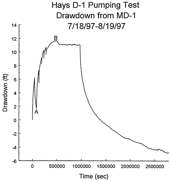
Figure 10A is a plot of the logarithm of time since pumping began versus drawdown for the entire pumping and recovery period at well MD-1. Figure 10B is the same data plotted in a time versus drawdown format. These two figures clearly show that the pump did not operate continuously for the entire pumping period. There were at least five times when the pump unexpectedly shut off as a result of electrical problems. There was also a decrease in pumping rate beginning at point B on Figure 10B that was most probably related to backpressure buildup in the city of Hays water distribution system into which the pumped water was discharged. Figures 10A and 10B show that there was significant recharge into the Dakota well field during the course of the test. This recharge is reflected in the stabilization of water levels in MD-1 both prior to and following the rate decrease at point B on Figure 10B. One component of this recharge was recovery from prior pumping activities in the well field. Although the negative drawdown (-4.9 ft) at the end of the monitoring period demonstrate the importance of the recovery process, leakage from surrounding low-permeability units was undoubtedly the most significant recharge mechanism.
Figure 10A--Plot of the logarithm of time since pumping began versus drawdown for the D-1 pumping test (drawdown measured with transducer in well MD-1).
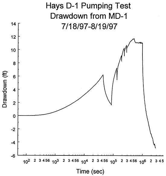
Figure 10B--Plot of the time since pumping began versus drawdown for the D-1 pumping test (drawdown measured with transducer in well MD-1; A and B defined in text).
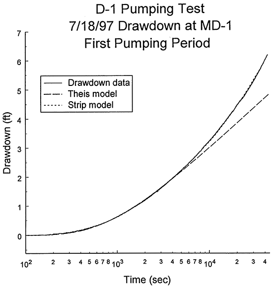
Significant variations in pumping rate and large amounts of recharge can introduce considerable uncertainty into the results of type-curve analyses. Thus, the primary focus of this analysis was on the first drawdown and recovery period (period ending at point A on Figure 10B). Figure 11 is a logarithm of time since pumping began versus drawdown plot for this period, during which a total of 4,001 transducer readings were acquired. Note that measurements of pumping rate indicated that the rate did not change significantly, and that 79 gpm would be a reasonable average rate for this first pumping period.
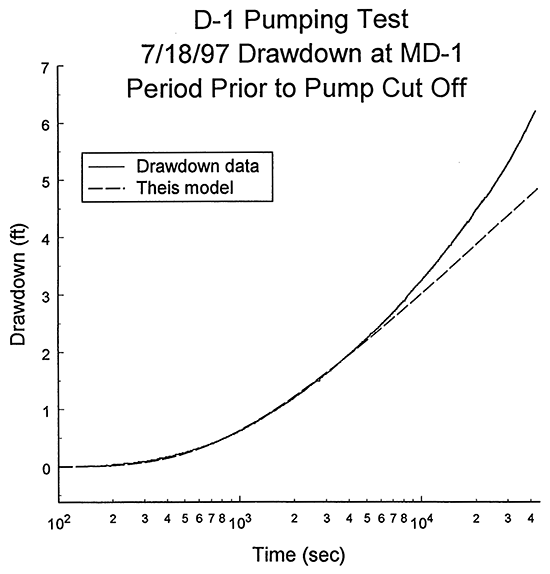
The first phase of the evaluation of the D-1 pumping test was to analyze the drawdown data with the Theis model. The concave-upward curvature of the drawdown plot of Figure 11 is an indication that lateral boundaries are affecting drawdown during the pumping period. Thus, as in the D-6 test, the strategy used with the Theis model was to initially analyze very early time data and then systematically extend the upper time limit of the data used in the analysis until boundary effects began to impact the results. The parameter estimates obtained from the analysis immediately prior to the appearance of boundary effects were considered the most reasonable estimates of transmissivity and storativity for the Dakota sands in the vicinity of wells D-1 and MD-1. Figure 12 displays the final Theis model resulting from this procedure. Note that the drawdown data begin to deviate from the Theis model at approximately 4,000 seconds after the start of pumping. The transmissivity and storativity estimates obtained from the analysis were 950 ft2/day and 1. 05X10-4, respectively. The first lateral boundary began to affect the drawdown data prior to the time at which the Cooper-Jacob semilog approximation would be valid, so the Theis model estimates could not be checked with the Cooper-Jacob method.
Figure 11--Plot of the logarithm of time since pumping began versus drawdown for the first portion of the D-1 pumping test (drawdown measured with transducer in well MD-1; interval prior to point A on Figure 10).
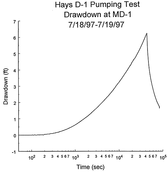
Figure 12--Logarithm of time since pumping began versus drawdown plot and the best-fit Theis type curve for the D-1 pumping test (drawdown measured with transducer in well MD-1; interval prior to point A on Figure 10).
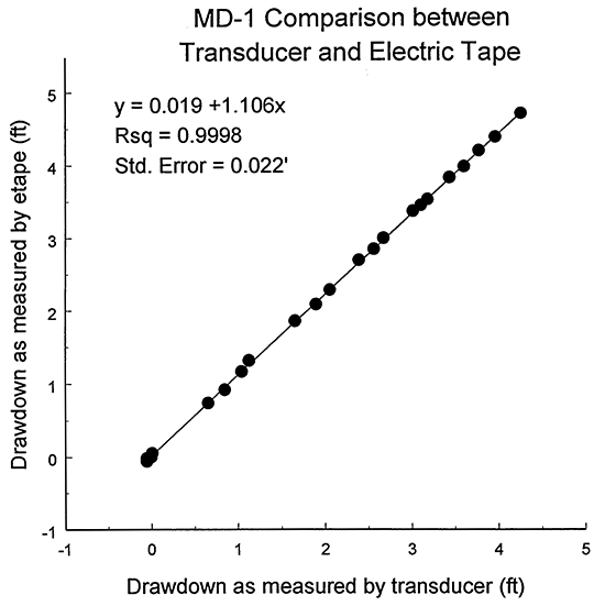
The estimates given in the previous paragraph were obtained using only the data from the pressure transducer in well MD-1. As discussed in the section on the D-6 test, transducer operation was checked in the field by comparing readings from the transducer with electric tape measurements taken at the same time. Figure 13 is a plot of drawdown as measured by the transducer in well MD-1 versus drawdown as measured in MD-1 with an electric tape. The slope of 1.106 for the best-fit line indicates that the calibration parameters for the transducer were producing a systematic underprediction of drawdown. This systematic under-prediction led to an overprediction of both transmissivity and storativity. Thus, the transmissivity and storativity estimates had to be corrected for the small errors in the calibration parameters. This correction was done by multiplying the parameter estimates determined for the Theis model by the inverse of 1.106 (0.904). The resulting transmissivity and storativity estimates were 859 ft2/day and 9.49 X 10⁻⁵, respectively. Note that these values are within 22% and 5%, respectively, of estimates obtained from an analysis of a 1992 pumping test performed at well D-1 using drawdown from well MD-1 (P. Allen Macfarlane, personal communication).
Figure 13--Calibration plot for transducer in well MD-1 (eqn. for best-fit line, and R2 and standard error of regression given in upper left-hand corner; electric tape measurements collected by P. Allen Macfarlane).
The second phase of the analysis process was to compare the drawdown data to theoretical plots produced by the strip model of Butler and Liu. The first task of this phase was to estimate the position of the closest lateral boundary. Figure 14 is a plot of the time since pumping began versus drawdown for the interval during which a lateral boundary first began to affect the drawdown data. The measured drawdown is plotted along with theoretical curves for drawdown in an infinite aquifer (Theis model) and for aquifers with single linear boundaries at different distances from the pumping well. In this case, the theoretical drawdown for a linear boundary at 1350 ft from the pumping well appears to most closely match the measured data. This theoretical drawdown was computed assuming that well MD-1 lies between the pumping well and the boundary on a line that is perpendicular to the boundary, and that transmissivity decreased by three orders of magnitude across the boundary (storativity did not change). This transmissivity contrast was the minimum contrast that could be used to reproduce the drawdown data. The slight deviation of the plot of measured drawdown from the theoretical curve at the upper end of the time range plotted on Figure 14 is possibly an indication that the contrast is larger than three orders of magnitude. Note that the exact distance of the boundary from the pumping well cannot be determined on the basis of this analysis. The distance of 1350 ft used here is actually the maximum possible distance to the boundary. The minimum distance to the boundary would occur for the case of a boundary perpendicular to the line connecting D-1 and MD-1, but lying on the opposite side of D-1 from MD-1. In this case, the boundary would be approximately 866 ft from the pumping well. Thus, the boundary is somewhere between 866-1350 ft from the pumping well, the exact distance depending on the location of the boundary relative to the position of the wells. For the purposes of the plots and discussions of this report, the maximum distance of 1350 ft is assumed.
Figure 14--Plot of the logarithm of time since pumping began versus drawdown for the D-1 pumping test with the best-fit Theis type curve and strip-model type curves for a single linear boundary (drawdown measured with transducer in MD-1; plot for interval of time during which first lateral boundary began to affect drawdown).
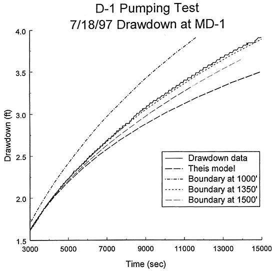
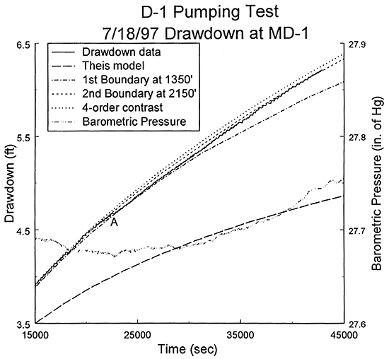
The second step of this phase of the analysis was to assess if there were any other lateral boundaries affecting the drawdown data. Figure 15 is a plot of the time since pumping began versus drawdown for the remainder of the pumping period after the interval of Figure 14. The measured drawdown is plotted along with theoretical curves for drawdown in an infinite aquifer (Theis model), an aquifer with a single linear boundary at 1350 ft from D-1, and an aquifer with two parallel linear boundaries on either side of D-1 at distances of 1350 and 2150 ft from the well. The systematic deviation from the single boundary case is a clear indication that a second boundary is affecting the measured drawdown. In this case, the theoretical drawdown for a second linear boundary at 2150 ft from the pumping well (2150 to 2634 ft depending on the position of D-1 and MD-1 relative to the boundary) appears to most closely match the measured data. This match, however, was not as good as seen with the first boundary. One reason for this is the shift in the drawdown plot in the vicinity of point A of Figure 15. This shift causes the data plot, which had been diverging from the single boundary case, to move back onto the single boundary case for another 2,000 seconds. After that time, the plot of the measured drawdown approaches the theoretical curve for a second boundary at 2150 ft. Figure 16 is the plot of Figure 15 with an additional theoretical curve for a transmissivity contrast of four orders of magnitude across the two boundaries. If the shift had not occurred, it appears that the drawdown plot might have converged on the four-order contrast curve. The exact cause of the shift at A is not known. It is possible that it is the product of a small decrease in pumping rate. Another explanation is undulations in the position of the two boundaries. Undoubtedly, the boundary between the Dakota sands and the surrounding low-permeability materials is not the abrupt vertical one assumed in the strip model of Butler and Liu. Thus, a more gradual transition from the Dakota sands to the low-permeability units could produce small deviations from the theoretical models. Fluctuations in barometric pressure could also be an explanation for the observed behavior. Figure 17 displays the curves of Figure 16 with the addition of the barometric pressure record from the transducer (electronic barometer) at MD-1. The fluctuations in barometric pressure were quite small for this time interval, so it is very unlikely that barometric pressure variations were the source of the shift. Thus, the most likely causes of the shift in the drawdown plot at point A are a small decrease in pumping rate and undulations in/a gradual transition across the boundaries between the Dakota sands and the surrounding low-permeability materials.
Figure 15--Plot of the time since pumping began versus drawdown for the D-1 pumping test with the best-fit Theis type curve and strip-model type curves for one and two linear boundaries (drawdown measured with transducer in MD-1; linear boundaries assumed to be parallel; A defined in text).
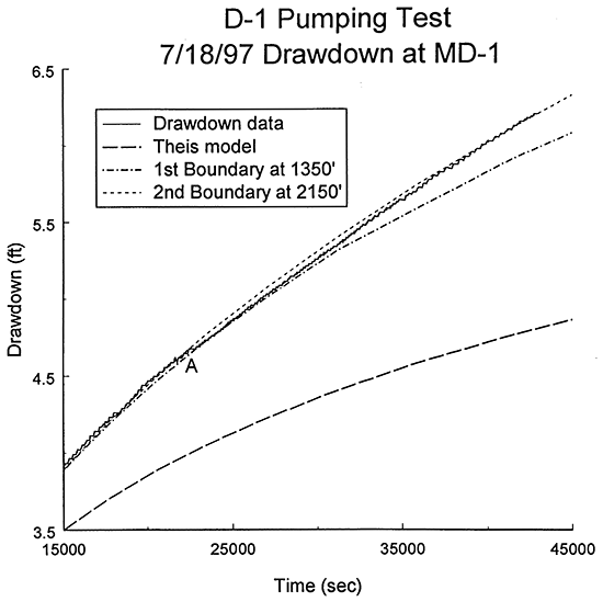
Figure 16--Plot of the time since pumping began versus drawdown for the D-1 pumping test with the best-fit Theis type curve and strip-model type curves for one and two linear boundaries (drawdown measured with transducer in MD-1; linear boundaries assumed to be parallel; A defined in text).
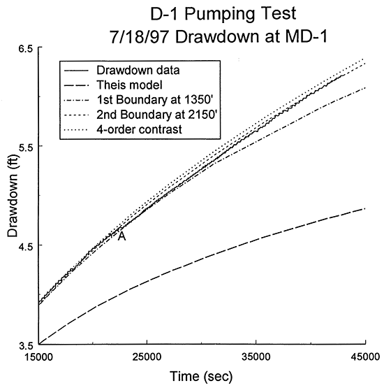
Figure 17--Plot of the time since pumping began versus drawdown for the D-1 pumping test with the best-fit Theis type curve, stripmodel type curves, and the barometric pressure record (drawdown measured with transducer in MD-1; barometric pressure measured with transducer at MD-1; A defined in text).
As stated earlier, the exact position of the boundaries relative to D-1 and MD-1 cannot be determined on the basis of this analysis. However, the width of the Dakota sands can be estimated with some confidence. In this case, the sands appear to be approximately 3500 ft in width. This width does not depend on assumptions regarding the position of the wells relative to the boundaries. Thus, if the minimum distance of 866 ft is used for the distance to the first boundary, the distance to the second boundary will be 2634 ft, but the width will still be 3500 ft.
Figure 18 displays the results of the second phase of the analysis of the MD-1 data. The relatively close match between the measured drawdown and the strip model of Butler and Liu is a further demonstration of the validity of the transmissivity and storativity estimates obtained in the first phase of the analysis.
Figure 18--Plot of the logarithm of time since pumping began versus drawdown for the D-1 pumping test with the best-fit Theis type curve and strip-model type curve for two linear boundaries (drawdown measured with transducer in MD-1; two linear boundaries are assumed to be parallel).
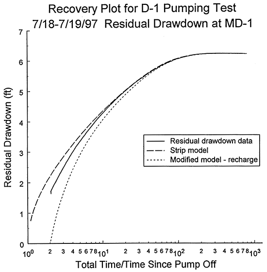
The final phase of the analysis of the MD-1 data was an examination of the recovery data. Figure 19 is a plot of the data in the format of the Theis recovery method (logarithm of the ratio of the total time since pumping began over the time since pump turned off versus residual drawdown). The large dashed line depicts the residual drawdown for the strip model of Butler and Liu using parallel linear boundaries at 1350 ft and 2150 ft from the pumping well with a transmissivity contrast of three orders of magnitude. As would be expected from theory, the model plot converges on a residual drawdown of zero as the time ratio goes to one. The measured residual drawdown, however, do not display this same convergence. Instead, as with the D-6 test, it appears that a negative residual drawdown would be obtained at a time ratio of one. The small dashed line on Figure 19 depicts the strip model modified, as was done in the analysis of the D-6 test, by assuming that if pumping had continued at D-1 drawdown would have stabilized and recharge would have been the source of all pumped water. The position of the plot of the residual drawdown between these two cases, which bound the range of possible recharge, is an indication that recharge accompanies pumping and recovery at D-1. In this case, a significant component of the recharge is undoubtedly a product of continuing recovery from the D-6 test and preceding pumping activity in the Dakota well field. Although the residual drawdown plot is closer to the unmodified strip model (i.e. no-recharge case), indicating that recharge is not the dominant mechanism during this time period, the stabilization of heads shown on Figures 10A-B in the later portions of the D-1 pumping test demonstrates that recharge from sources other than recovery from previous pumping activity eventually does play the dominant role in the D-1 test. As with the D-6 test, however, it is difficult to determine the source of that recharge. Note that the close match between the residual drawdown measurements and the theoretical residual drawdown computed with the strip model (unmodified case) above a time ratio of ten is a further demonstration of the validity of the parameter estimates obtained with the Theis model in the first phase of the analysis.
Figure 19--Plot of the log of the ratio of the total time since pumping began over the time since pump was cut off versus the residual drawdown for the D-1 pumping test with two strip-model type curves (residual drawdown measured with transducer in MD-1; modifications to the strip model described in text).
An additional check on the results of the analysis of the first pumping and recovery periods was performed using data from the second pumping period. The second pumping period began at approximately 23.42 hours (84,298 secs) after the start of the D-1 test, and ended at 35.40 hour after the start of the D-1 test. The duration of the second pumping period was approximately 11.98 hours (43,145 secs). This duration estimate should be considered a lower bound on the time of pumping because there was some uncertainty about the exact start and stop times for this second pumping period. The pumping rate was approximately the same as for the first period (79 gpm), although the rate was 5-10% higher in the early portions of this period.
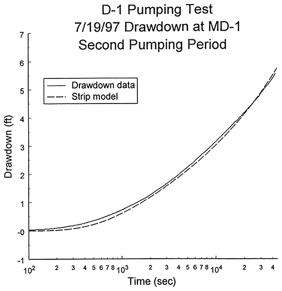
Figure 20 is a logarithm of time since pumping began versus drawdown plot for this second pumping period. Both the measured drawdown and the theoretical drawdown computed with the strip model using the parameters determined from the analysis of the first pumping period are shown. The relatively close match between the measured and theoretical drawdown is a further demonstration of the validity of the estimates determined in the analysis of the first pumping period. The differences between measured and theoretical drawdown seen shortly after the start of pumping are probably a product of uncertainty regarding the exact start time of the test, and an initial pumping rate that was greater than the average rate for the test. The differences seen in the later portions of the test are probably a product of recovery from pumping activity prior to the D-1 test and recharge from the same sources that produce the eventual stabilization of drawdown later in the D-1 test (see Figure 10B). Although similar plots could have been produced for all the pumping periods in the D-1 test, little additional insight would have been gained into the hydraulic properties and lateral boundaries of the Dakota sands in the vicinity of wells D-1 and MD-1. Uncertainty regarding the start and end times for these pumping periods increases because of the larger time interval (8 minutes for the most part) used to collect data in these periods. When this is coupled with increasing recharge and further uncertainty about pumping variations in the vicinity of point B of Figure 10B, it is difficult to gain additional insight regarding the properties of the Dakota sands. Thus, the type-curve analysis of the D-1 pumping test concluded with the comparison of measured and theoretical drawdown for the second pumping period.
Figure 20--Plot of the logarithm of time since pumping began versus drawdown for the second pumping period of the D-1 pumping test with the strip-model type curve for two linear boundaries (drawdown measured with transducer in MD-1; two linear boundaries are assumed to be parallel).
In summary, there are six major findings of the analysis of the MD-1 data: 1) 859 ft2/day and 9.49 X 10⁻⁵ appear to be reasonable estimates for the transmissivity and storativity, respectively, of the Dakota sands in the vicinity of wells D-1 and MD-1; 2) there appears to be a linear boundary separating the Dakota sands from surrounding units of lower permeability at a maximum distance of 1350 ft from well D-1; 3) there appears to be a second linear boundary separating the Dakota sands from surrounding units of lower permeability at a minimum distance of 2150 ft from well D-1; 4) the Dakota sands appear to be approximately 3500 ft in width in the vicinity of wells D-1 and MD-1; 5) the decrease in transmissivity across the boundaries appears to be at least 3-4 orders of magnitude; and 6) there appears to be a significant amount of recharge into the Dakota sands during pumping at D-1. Al though some of this recharge was a product of recovery from previous pumping activities, the most significant component was undoubtedly induced by pumping at well D-1.
The parameter estimates obtained from the analyses described in the previous sections are for vertically integrated quantities. Since the numerical model of the well field requires estimates of the average hydraulic conductivity (K) of the Dakota sands as input, the transmissivity values obtained from the type curve analyses must be converted into K values. In order to perform this conversion, estimates of the aquifer thickness in the vicinity of the two well pairs are needed. Tables 1 and 2 indicate that there is considerable variability in sand thickness in the vicinity of both well pairs. Using the two thicknesses for each well pair as bounds for the thickness of the Dakota sands in the vicinity of those wells, K estimates of 9.3-19.5 ft/day and 14.6-23.2 ft/day are obtained for the vicinity of wells D-6 and D-1, respectively. In order to compare the average K estimates from the Hays well field with values obtained at other sites in the Dakota aquifer, the Hays estimates must be converted to either permeability estimates or to the standard laboratory conditions for reporting hydraulic conductivity values (pure water at 15.6 deg. C (Fetter, 1994) ). Since most other Dakota estimates are reported as hydraulic conductivity values, the latter approach was used here. The average water temperature and chloride concentration measured during the pumping tests were approximately 21.5 deg. C and 570. mg/l, respectively. Considering only the temperature correction, the K ranges for the vicinity of wells D-6 and D-1 convert to ranges of 8.0-16.8 ft/day and 12.6-20.0 ft/day, respectively. Laboratory data detailing viscosity and density changes as a function of sodium chloride concentration (Weast, 1976) indicate that a correction for salinity would change K values a negligible amount for these tests. Thus, a salinity correction was not deemed necessary. Note that the K ranges obtained through these analyses are consistent with other estimates obtained for the Dakota aquifer in Kansas (e.g., Macfarlane et al., 1990).
Two multi-day pumping tests were performed by the Kansas Geological Survey in the Dakota well field of the city of Hays in Ellis County, Kansas in July of 1997. The major objective of these tests was to obtain information about the hydraulic and geochemical responses of the well field to extended periods of pumping. This report described the type curve analyses that were performed on the drawdown data from the observation well closest to each pumping well. The purpose of these analyses was to obtain parameter estimates for input to a numerical model of the well field. Table 3 summarizes the results of these analyses. The hydraulic property estimates are quite reasonable for the Dakota sands and are in good agreement with the results of 1992 tests performed at the same wells. The width estimates are in reasonable agreement with maps of the Dakota sand thickness constructed from well logs. The effects of recharge were quite pronounced in the later portions of both pumping tests. Although it is not possible to precisely specify the source of that recharge on the basis of these analyses, leakage from adjacent low-permeability units is probably the most significant recharge mechanism.
Table 3--Results of type-curve analyses of July 1997 pumping tests in the Dakota well field of the city of Hays.
| Test Name |
T1 | S2 (X 10-5) |
Average K3 |
Sand Width4 |
Evidence of Recharge? |
|---|---|---|---|---|---|
| D-1 | 859 | 9.49 | 14.6-23.2 | 3500 | Yes5 |
| D-6 | 584 | 6.95 | 9.3-19.5 | 6000 | Yes5 |
| 1 - transmissivity, units are ft2/day 2 - storage coefficient, dimensionless parameter 3 - average hydraulic conductivity, units are ft/day 4 - units are ft 5 - recharge evident on both drawdown and residual drawdown plots, source of recharge unknown |
|||||
Bohling, G.C., C.D. McElwee, J.J. Butler, Jr., and W.Z. Liu. 1990. User's Guide to Well Test Design and Analysis with SUPRPUMP Version 1.0: Kansas Geological Survey, Computer Program series 90-3, 95 pp.
Bohling, G.C. and C.D. McElwee. 1992. SUPRPUMP: An interactive program for well test analysis and design: Ground Water, v. 30, no. 2, pp. 262-268.
Butler, J.J., Jr. 1990. The role of pumping tests in site characterization: Some theoretical considerations: Ground Water, v. 28, no. 3, pp. 394-402.
Butler, J.J., Jr. 1997. The Design, Performance, and Analysis of Slug Tests: Lewis Pub., Boca Raton, 252 pp.
Butler, J.J., Jr. and W.Z. Liu. 1991. Pumping tests in non-uniform aquifers - the linear strip case: Jour. of Hydrology, v. 128, pp. 69-99.
Fetter, C.W. 1994. Applied Hydrogeology: Macmillan, New York, 691 pp.
Kruseman, G.P. and N.A. de Ridder. 1990. Analysis and Evaluation of Pumping Test Data: ILRI, The Netherlands, pub. 47, 377 pp.
Macfarlane, P.A., D.O. Whittemore, M.A. Townsend, J.H. Doveton, V.J. Hamilton, W.G. Coyle, III, A. Wade, G.L. Macpherson, and R.D. Black. 1990. The Dakota Aquifer Program: Annual report, FY89. Kansas Geological Survey, Open-File Rept. 90-27, 302 pp. [available online]
Streltsova, T.D. 1988. Well Testing in Heterogeneous Formations: John Wiley, New York, 413 pp.
Weast, R.C. (ed.). 1976. CRC Handbook of Chemistry and Physics: CRC Press, Cleveland, OH, pp. D252-D253.
Kansas Geological Survey, Geohydrology
Placed online Feb. 25, 2015
Comments to webadmin@kgs.ku.edu
The URL for this page is http://www.kgs.ku.edu/Hydro/Publications/1998/OFR98_15A/index.html