Kansas Geological Survey, Open-file Report 2005-19
Part of the Phreatophyte Research Project Project
by
James J. Butler, Jr., Donald O. Whittemore, and Gerard J. Kluitenberg
KGS Open File Report 2005-19
Prepared for thr Kansas Water Office
July 2005
Project: Ground Water Assessment in Association with Salt Cedar Control
Duration: August 16, 2004 to June 30, 2005
Lead Investigator and Affiliation: James Butler, Kansas Geological Survey
Associated Investigators and Affiliations: Gerard Kluitenberg, Kansas State University, Donald Whittemore, Kansas Geological Survey
KWO Contract Number: 05-114; Total Funding: $20,637
The primary objective of the work described here was to use water-table fluctuations to estimate the impact of various salt-cedar control activities on the ground-water resources of the Cimarron River alluvial aquifer at a site in Clark County. Previous work by this KGS/KSU research team has shown that diurnal fluctuations in the water table can be utilized both as a diagnostic indicator of phreatophyte activity and for quantifying ground-water consumption by phreatophytes. This contract was developed to extend the work of the research group to exploit an opportunity presented by a Kansas Alliance of Wetlands and Streams (KAWS) demonstration project focused on investigating the effectiveness of various salt-cedar control measures. Funding for this contract was provided by the Kansas Water Plan through the Kansas Water Office.
The KAWS demonstration project is being carried out in an area of salt-cedar infestation along the Cimarron River south of Ashland. Four experimental plots were established in pasture on the north side of the Cimarron River. One plot is used for monitoring background (unaltered) conditions, while the other three plots are for application of different salt-cedar control measures. Application of control measures began in mid-March of 2005 and is continuing.
Six shallow wells were installed in three of the experimental plots in August 2004. All wells have submersible pressure sensors to allow monitoring of water levels through time. Water-level data collected in the late summer and early fall of 2004, prior to any control activities and prior to salt-cedar dormancy, clearly demonstrate that the magnitude of the diurnal water-table fluctuations observed at a well is highly dependent on the vitality of the phreatophyte community in the vicinity of that well. Thus, the strategy of using water-table fluctuations to assess ground-water savings achieved from control activities appears to have considerable potential at this site.
Other hydrologic data are being collected as part of this work. A weather station was installed in October 2004 to monitor meteorological conditions and provide estimates of the potential for evapotranspiration. A neutron-probe access tube was installed adjacent to each well in August 2004 to monitor the moisture content above the water table.
The application of salt-cedar control measures is ongoing. As of this report, plots have been cleared of salt cedar except for circles around each well. Those circles will be gradually reduced until all vegetation is eliminated in July of 2005. After all the salt cedar and other phreatophytes have been removed, monitoring will continue in order to evaluate the ground-water savings gained through the control activities. However, short-term monitoring will only provide information about short-term gains. Longer-term monitoring is critical for assessing the ultimate ground-water savings gained through the control activities. Modest funding for that additional monitoring has been requested from the Kansas Water Office.
Consumption of ground water by phreatophytes in riparian corridors is thought to be one factor responsible for stream-flow reductions in the Cimarron Basin and elsewhere in western Kansas. Extensive phreatophyte-control measures, primarily focusing on invasive species such as salt cedar (Tamarix spp.) and Russian olive (Elaeagnus angustifolia), are being considered in response to concerns about the impact of phreatophytes on surface- and ground-water resources. At present, there is no generally accepted means of quantifying the ground-water savings that might be gained through these control measures. Recently, a team of Kansas Geological Survey (KGS) and Kansas State University (KSU) researchers have shown that diurnal fluctuations in the water table can be utilized both as a diagnostic indicator of phreatophyte activity and for quantifying ground-water consumption by phreatophytes (Butler et al., in review). This Kansas Water Office (KWO) contract was directed at extending that previous work to assess the use of water-table fluctuations as a tool for quantifying ground-water savings achieved through phreatophyte control measures.
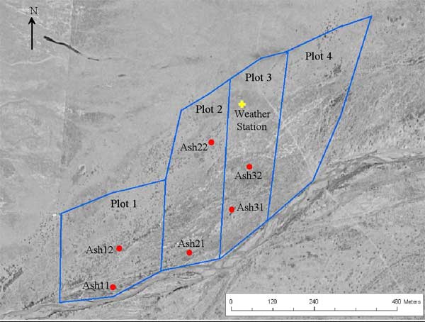
The KWO contract was developed to exploit an opportunity presented by a Kansas Alliance of Wetlands and Streams (KAWS) demonstration project focused on investigating the effectiveness of various salt-cedar control measures. The demonstration project is being carried out in an area of salt-cedar infestation along the Cimarron River south of Ashland, Kansas (Figure 1). Four experimental plots have been established on the north side of the Cimarron River on pasture of the Arnold Ranch (Figure 2). One area (Plot 1) is to remain unaltered during the project, while different salt-cedar control measure will be applied in the other three areas. The salt cedar will be cut and chemically treated in Plot 2, repeatedly cut in Plot 3, and cut and burned in Plot 4.
Figure 1--Location map of the Ashland Research Site (ARS). The Ashland Research Site is the KGS designation for the area on the Arnold Ranch in which the work described in this report was carried out.
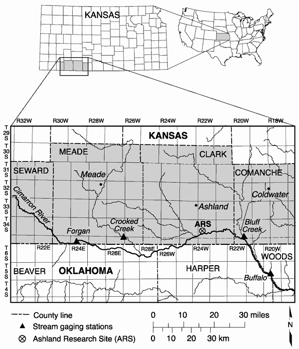
Figure 2--Aerial photo of Ashland Research Site with locations of the experimental plots, monitoring wells, and weather station.
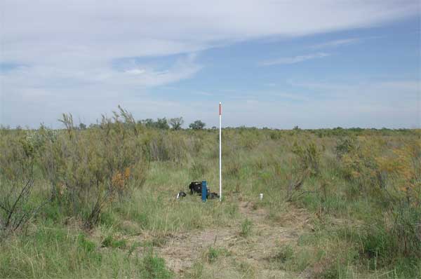
The Arnold Ranch has been owned and operated by the Arnold family since its establishment in the late 1800s. According to the Arnold family, salt cedar was first noted on their ranch after the flood of 1939. The salt cedar sprouted on the wet sand deposited by that flood and its distribution across the area has changed little since then. Dave Arnold clear cut Plots 1-3 in the fall of 1996. The heterogeneous pattern of salt cedar and Russian olive growth observed in Plots 1-3 at the start of this project (mid-August 2004) was not a function of how the plots were cut in 1996. That distribution was most likely a reflection of spatial variations in underlying soil conditions.
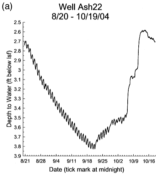
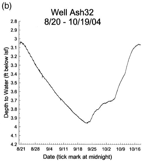
In the reporting period for this contract, six wells equipped with submersible pressure sensors were installed in Plots 1-3 in order to monitor water-table responses in the vicinity of the most common phreatophyte communities at the site (wells were not placed in Plot 4 because of concerns about possible well damage from the planned burning). A neutron-probe access tube was emplaced adjacent to each well so that water content in the vadose zone (interval between the water table and the land surface) could also be measured. A weather station was installed on the north end of Plot 3 to monitor meteorological conditions and provide estimates of the potential for evapotranspiration. Water-level data collected in the late summer and early fall of 2004, prior to any control activities and prior to salt-cedar dormancy, clearly demonstrate that the magnitude of the diurnal water-table fluctuations observed at a well is highly dependent on the apparent vitality of the phreatophyte community in the vicinity of that well (Figures 3a-b). Thus, the initial data indicate that the strategy of using water-table fluctuations to assess ground-water savings gained from control activities appears to have considerable potential at this site.
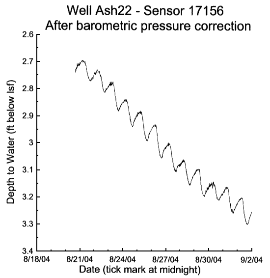
Figure 3--Depth to water recorded in two wells at the Ashland Research Site prior to application of salt-cedar control measures. Well Ash22 (a) is located in an area of vigorous salt cedar growth, while well Ash32 (b) is located in an area of stunted salt cedar. Note that the length of the interval represented by the y-axis is the same for both plots.
Application of salt-cedar control measures began in March 2005 (Figures 4a-c). At that time, plots 2-4 were clear cut except for circles ranging from 70-100 ft in radius about the four monitoring wells in Plots 2 and 3. The radii of those circles of vegetation were reduced to 45 ft at three of the four wells on June 3, 2005. The vegetation was completely cleared about well Ash32 on June 3 because of the lack of any plant-induced water-table responses at that well since the start of monitoring in August 2004 (Figure 3b). The circles at the other three wells in Plots 2 and 3 were reduced to 22 ft on June 27, 2005. Two weeks later, all plants except one will be cut in the three remaining circles. In approximately another two weeks, the final plant in each plot will be removed. After the control measures have been fully applied, water-level data from the treated plots will be compared to data from the untreated area (Plot 1). That comparison should enable quantification of reductions in ground-water consumption produced by those measures. Note that a number of tasks not funded by this contract were also performed by the KGS/KSU research team in order to increase the value of the project results. For example, data on vegetation within the experimental plots were not obtained as originally planned by cooperators on the KAWS project. Thus, the research team decided to collect vegetation data on its own as the circles about the wells were reduced below 45 ft in radius. That vegetation inventory is ongoing so the results will be presented in a subsequent project report.
Figure 4a--Aerial photo of Ashland Research Site with boundaries of vegetation circles remaining after mid-March 2005 and June 3, 2005, cuttings (circle boundaries recorded with handheld GPS unit; vegetation completely cleared around well Ash32 on June 3);
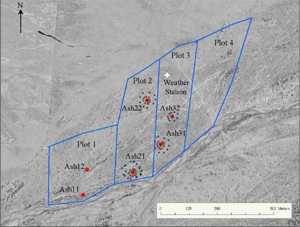
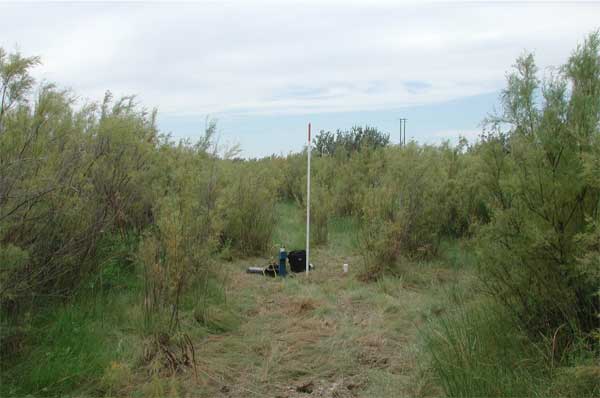
Figure 4b--Photo (6/16/05) of vegetation circle around well Ash22 following June 3rd cutting (view looking north, ATV on left for scale, pole visible at center of plot is 8.5 ft in height; note remnants of cut salt cedar in foreground);
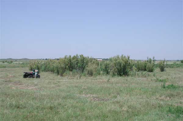
Figure 4c--Photo (6/16/05) of large salt cedar that will remain as the single plant near well Ash22 (red tape used to indicate plants that should remain following next cutting to reduce the circle to 22 ft in radius).
The following report is divided into two main sections: 1) Installation of the Monitoring Network; and 2) Data Management, Processing, and Preliminary Analysis. The first section describes approaches used to design and install the monitoring wells and the neutron-probe access tubes, and the equipment utilized to monitor hydrologic and meteorological conditions at the site. The second section describes data management and processing procedures, presents a sample of the water-level data that have been collected in the project, discusses some problems affecting the quality of the water-level data, and summarizes the procedures for and initial results from the neutron logging.
The first four tasks listed in the scope of work outlined in the KWO contract involved installation of the monitoring network. Those tasks and the date on which they were completed are as follows:
Each of these tasks is described in this section.
As soon as the KWO contract was formally activated (August 16, 2004), KGS and KSU personnel traveled to the Arnold Ranch to install the monitoring wells and neutron-probe access tubes. This installation work was done August 17-20, 2004. Well locations were based on a qualitative survey of vegetation patterns in each plot by members of the KGS/KSU research team; an attempt was made to place wells in the vicinity of typical phreatophyte groupings found over the area. Prior to well installation, six direct-push electrical-conductivity (EC) profiles were performed to assess the water-table position and shallow stratigraphy at each well site. At each location, EC logging (see Butler et al. [1999] and Schulmeister et al. [2003] for a description of direct-push EC logging) was performed to a depth of approximately 23 ft below land surface (lsf) with the KGS Geoprobe machine. After review of the EC log, a 2-in ID PVC well was installed in the EC hole using the Geoprobe machine. The screened interval of all the wells was relatively long to allow specific conductivity profiling (an activity not funded by this contract) to be carried out. An additional factor influencing the length of the screened interval was the uncertainty regarding the vertical range over which the water table might vary through time. In the absence of any data, the decision was made to err on the side of caution and use relatively long screens. Note that a long screened interval may serve as a preferential flowpath to bring water up to meet the demands of the salt cedar and other phreatophytes, so it may diminish the observed water-table fluctuations. We are currently examining the potential of this mechanism to introduce bias into the collected data. Installation was completed by placing a metal surface casing over the PVC well. Following installation, the well was pumped and surged using a suction pump. When the turbidity of the water no longer changed after surging, a water sample was taken and placed on ice (note that water sampling was not an activity funded by this contract).
A neutron-probe access tube was installed a few feet from each well. A pilot hole of a diameter slightly smaller than the outer diameter of the neutron-probe access tube was first made with the Geoprobe machine, after which the tube was pounded into the hole using a cathead arrangement. Neutron-probe access tubes were constructed from 1.5-in Schedule 40 PVC tubing (1.90-in OD). At one end, the access tubes were fit with a well point to allow insertion into the soil and to prevent water entry. The well points were fabricated (Environmental Manufacturing Inc.) from PVC rod and threaded onto the end of the access tubes. This threaded connection was further secured with PVC cement. Approximately 0.5 ft of tubing remained above the soil after installation. Local soil material was packed around the tube at the soil surface to provide a seal. After an access tube was installed, it was closed with a rubber stopper to prevent water entry from above. A cover fabricated from a PVC end-cap and a short length of PVC tubing were also placed over each tube to further limit water entry.
A description of each well site is given in the following subsections. Table 1 provides well-completion information and associated data for each well. Note that in the absence of a nearby surveyed benchmark, the top of casing (TOC) elevation for each well was measured with respect to TOC at well Ash11.
Table 1--Well-completion details and associated information for monitoring wells (all wells constructed with 2-in ID Sch40 PVC casing and screen (10-slot [0.01 in]); latitude and longitude of wells determined with high-accuracy KGS GPS surveying system, relative TOC elevations determined with same system; lsf and wrt are abbreviations for "land surface" and "with respect to", respectively).
| Well | Total depth from lsf (ft) |
TOC above lsf (ft) |
Screened interval wrt lsf (ft) |
Sump interval wrt lsf (ft) |
Sensor type and serial number |
Lateral distance to neutron-probe access tube (ft) |
Latitude (deg) |
Longitude (deg) |
Elevation of TOC above Ash11 TOC (ft) |
Height of pole above lsf (ft) |
|---|---|---|---|---|---|---|---|---|---|---|
| Ash11 | 21.11 | 1.7 | 3.29-18.06 | 18.06-21.11 | Troll 9000--#31947 | 3.35 | 37.0439 | 99.7569 | 0.000 | 8.33 |
| Ash12 | 21.12 | 1.69 | 3.29-18.08 | 18.08-21.12 | miniTroll--#15936 baroTroll--#16977 |
4.20 | 37.0449 | 99.7567 | 3.251 | 8.33 |
| Ash21 | 21.16 | 1.64 | 3.32-18.09 | 18.09-21.16 | miniTroll--#17162 | 4.1 | 37.0448 | 99.7544 | 1.193 | 7.17 |
| Ash22 | 21.07 | 1.73 | 3.32-18.04 | 18.04-21.07 | miniTroll--#17156 | 4.49 | 37.0477 | 99.7537 | 1.071 | 8.5 |
| Ash31 | 21.17 | 1.65 | 3.32-18.11 | 18.11-21.17 | miniTroll--#17201 | 4.72 | 37.046 | 99.753 | 0.021 | 7.33 |
| Ash32 | 21.11 | 1.69 | 3.19-17.97 | 17.97-21.11 | miniTroll--#16940 baroTroll--#17026 |
4.72 | 37.0471 | 99.7525 | 0.951 | 8.25 |
Well Ash11
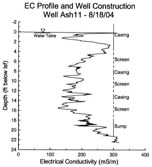
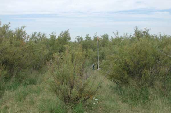
This well site is located near the south edge of Plot 1 in a low-lying area of dense salt cedar near the Cimarron River (Figure 5a). The water table was within 0.3 ft of the land surface at the time of installation and remained close to the surface for most of the monitoring period due to the proximity of the Cimarron River. Figure 5b displays the EC log obtained at the site and relevant well-completion information. The well is screened from 3.3-18.1 ft below lsf. It appears that the top of the screen is in a zone with some clay. The interval from 6-16 ft, however, appears to have little clay and is thought to consist primarily of sand. The relatively high EC (for sand) values in that interval are a product of the high specific conductance of the ground water (sample collected 8/18/04: 10,000 μS/cm at 25 deg C = 1,000 mS/m in units of EC log) with very little matrix contribution.
Figure 5--Photograph (a) and EC log (b) for Ash11 well site (see Table 1 for further well information; photograph taken on 8/31/04).
Well Ash12
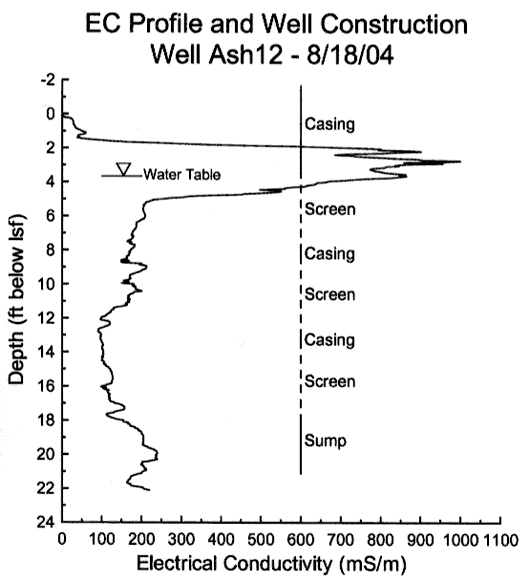
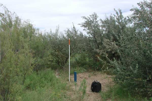
This well site is located near the center of Plot 1 on a terrace above the Cimarron River in the densest growth of salt cedar observed on the site (Figure 6a). The water table was 3.7 ft from the land surface at the time of installation. Figure 6b displays the EC log obtained at the site and relevant well-completion information. The well was screened from 3.3-18.1 ft below lsf. It appears that the top of the screen is in the lower portions of a clay-rich zone that extends from 1.5-5 ft below lsf. The interval from 6-11 ft is characterized by an approximately constant EC and is thought to consist primarily of sand with small amounts of fine material. The relatively high (for sands) EC values in that interval are primarily a product of the high specific conductance of the ground water (sample collected 8/18/04: 7,740 μS/cm at 25 deg C = 774 mS/m in units of EC log). Later specific conductance profiling found that the drop in EC at about 11 ft is not caused by a change in fluid EC. The most likely cause of that drop is a decrease in porosity and/or clay content.
Figure 6--Photograph (a) and EC log (b) for Ash12 well site (see Table 1 for further well information; photograph taken on 8/31/04).
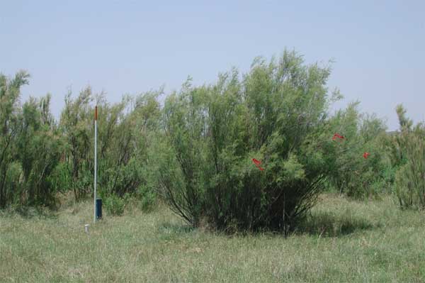
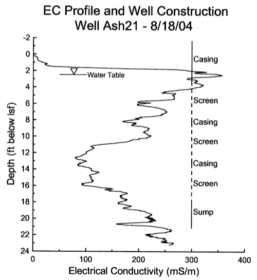
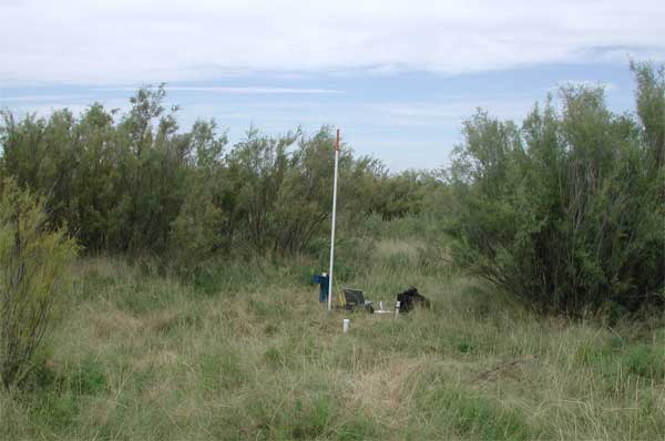
Well Ash21
This well site is located near the southern boundary of Plot 2 on the first terrace above the Cimarron River. The well is in an area of salt cedar and Russian olive (Figure 7a) that occur in a thin band across the southern portions of Plot 2; the Russian olive at the back right of the clearing in Figure 7a was one of the largest trees found on the four plots. The water table was 2.4 ft from the land surface at the time of installation. Figure 7b displays the EC log obtained at the site and relevant well-completion information. The well was screened from 3.3-18.1 ft below lsf. It appears that the top of the screen is in a zone with some clay that extends from 1.5-4.5 ft below lsf. The interval from 5.5-10 ft is thought to be sand. The relatively high (for sands) EC values in that interval are primarily a product of the high specific conductance of the ground water (sample collected 8/19/04: 8,890 μS/cm at 25 deg C = 889 mS/m in units of EC log) with minor matrix contribution. Later specific conductance profiling found that the lower EC values from 11-16 ft are not caused by a change in fluid EC. The most likely causes of that drop are a decrease in porosity and/or clay content similar to that suspected at well Ash12. Similarly, the increase in EC from 16-18 ft is not caused by a change in fluid EC and is most likely a result of an increase in porosity and/or clay content.
Figure 7--Photograph (a) and EC log (b) for Ash21 well site (see Table 1 for further well information; photograph taken on 8/31/04).
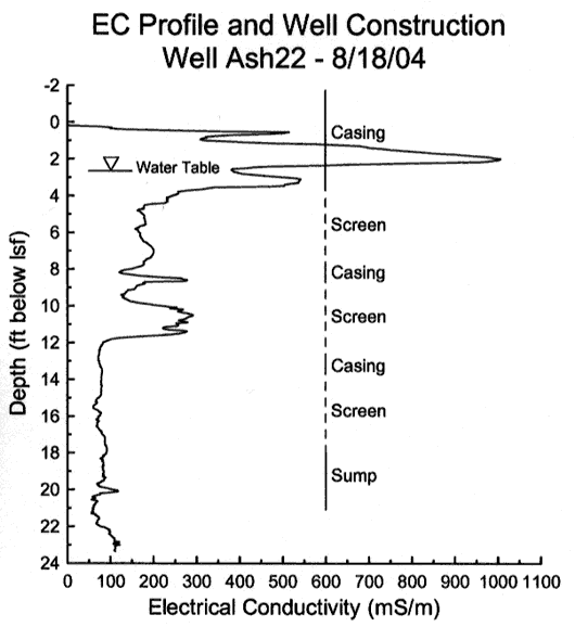
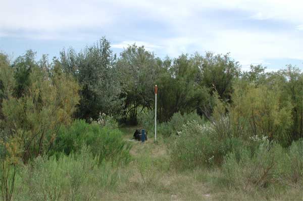
Well Ash22
This well site is located in the northern half of Plot 2 in an area of large thriving clumps of salt cedar (Figure 8a). These salt cedar are the largest and healthiest looking in the four plots. The water table was 2.7 ft from the land surface at the time of installation. Figure 8b displays the EC log obtained at the site and relevant well-completion information. The well was screened from 3.3-18.0 ft below lsf. There are three distinct segments to the EC log. The top of the screen appears to be in a zone of high EC that extends from 0.5-4 ft below lsf. The interval from 4-11.5 ft is characterized by relatively constant EC and is thought to consist primarily of sand with some clay. The relatively high (for sands) EC values in that interval are a product of the high specific conductance of the ground water (sample collected 8/19/04: 5,100 μS/cm at 25 deg C = 510 mS/m in units of EC log) with additional matrix contribution. Specific conductance profiling found that the lower EC values below 11.5 ft are not caused by a change in fluid EC. The most likely cause of that drop is a decrease in porosity and/or clay content similar to that suspected at wells Ash12 and Ash21.
Figure 8--Photograph (a) and EC log (b) for Ash22 well site (see Table 1 for further well information; photograph taken on 8/31/04).
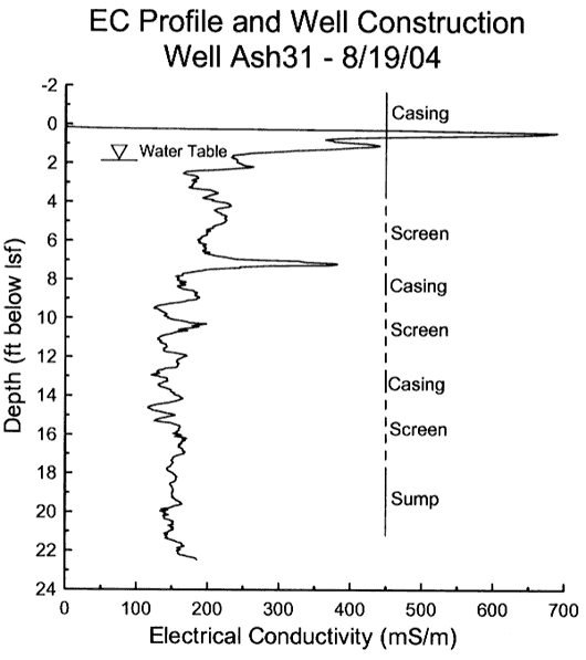
Well Ash31
This well site is located in a low-lying area in the southern half of Plot 3. The site is in a thin band of salt cedar and Russian olive (similar to well Ash21) that extends across Plot 3 (Figure 9a). The water table was 1.9 ft from the land surface at the time of installation. Figure 9b displays the EC log obtained at the site and relevant well-completion information. The well was screened from 3.3-18.1 ft below lsf. There are three distinct segments on the EC log. There is a zone of high EC that extends from the surface to about 1.5 ft below lsf. The top of the screen is in an interval that extends 2-7.5 ft below lsf that is characterized by a relatively constant EC and is thought to consist primarily of sand with some finer material. The relatively high (for sands) EC values in that interval are a product of the high specific conductance of the ground water (sample collected 8/19/04: 7,000 μS/cm at 25 deg C = 700 mS/m in units of EC log) with some matrix contribution. Specific conductance profiling found that the lower EC values below 7.5 ft are not caused by a change in fluid EC. The most likely cause of that drop is a decrease in porosity and/or clay content similar to that suspected at wells Ash12, Ash21, and Ash22. The EC decrease, however, is smaller than that observed at the other wells.
Figure 9--Photograph (a) and EC log (b) for Ash31 well site (see Table 1 for further well information; photograph taken on 8/31/04).
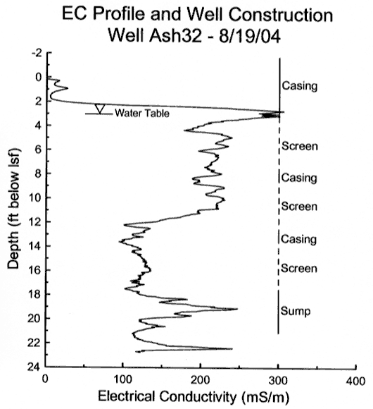
Well Ash32
This well site is located in the middle of Plot 3 in a zone of diminutive and sickly looking salt cedar that stretches across all four plots (Figure 10a). The water table was 3.0 ft from the land surface at the time of installation. Figure 10b displays the EC log obtained at the site and relevant well-completion information. The well was screened from 3.2-18.0 ft below lsf. There are four distinct segments on the EC log. A zone of very low EC, most likely indicative of dry sand, extends from the surface to a depth of 2 ft. A zone of higher EC caused by salt accumulation and/or a higher clay content extends from 2 to 3.5 ft below lsf with the top of the screen near the bottom of that zone. A zone of relatively constant EC extends from 3.5 to 11 ft below lsf and is thought to consist primarily of sand with lesser amounts of clay. The relatively high (for sands) EC values in that interval are a product of the high specific conductance of the ground water (sample collected 8/19/04: 8,260 μS/cm at 25 deg C = 826 mS/m in units of EC log) with some matrix contribution. A zone of lower EC extends to the bottom of the screen. Specific conductance profiling found that the lower EC values below 11 ft are not caused by a change in fluid EC. The most likely cause of that drop is a decrease in porosity and/or clay content similar to that suspected at all the other wells except Ash11.
Figure 10--Photograph (a) and EC log (b) for Ash32 well site (see Table 1 for further well information; photograph taken on 8/31/04).
All wells except Ash11 have an integrated pressure-transducer and datalogger unit submerged in the water column (30 psi absolute-pressure miniTroll, In-Situ, Inc.). This unit measures and records the pressure exerted by the overlying column of water and the atmosphere. Ash11 has a more sophisticated sensor (Troll 9000, In-Situ, Inc.) that measures the specific conductance and temperature of the ground water, as well as the pressure exerted by the overlying column of water and the atmosphere. Pressure readings are taken every 15 minutes in all wells and checked periodically with manual depth-to-water measurements (biweekly during the summer months and bimonthly otherwise). The temperature and specific conductance of the ground water at well Ash11 are measured at that same 15-minute interval and sensor operation is checked periodically using a hand-held specific-conductance and temperature meter (Model 30 Conductivity and Temperature Probe, YSI). As of the end of this reporting period, all sensors appeared to be performing well.
Absolute-pressure sensors were used in the wells instead of gage-pressure sensors in order to prevent sensor damage (via water movement down the vent tube of a gauge-pressure sensor) in the case a well is overtopped during high river stages. The Cimarron River overtopped Ash11 at least twice during this reporting period and reached the base of well Ash31 on at least one occasion (observations by the research team and Dave Arnold), demonstrating the need for absolute-pressure sensors in those wells. In order to compute the height of the overlying column of water (and thus the position of the water table) from the absolute-pressure measurement, the atmospheric-pressure component of that measurement must be removed. Atmospheric pressure is measured at the same 15-minute interval using two on-site barometers (baroTroll, In-Situ, Inc.) placed in the air column above the water table in wells Ash12 and Ash32. Figures 11a-b display records from the sensor in well Ash22 prior to and after the barometric pressure correction, respectively. Because of unanticipated problems with the barometers at wells Ash12 and Ash32 discussed in a later section, an additional barometer was placed in the weather station near the end of the reporting period.
Figure 11a--Absolute-pressure record from sensor (17156) in the water column in Ash22;
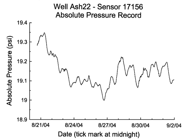
Figure 11b--Depth to water at well Ash22 calculated after atmospheric-pressure component is removed from Ash22 sensor using barometer (sensor 16977) in air column at well Ash12.
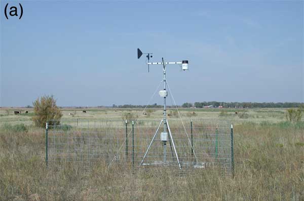
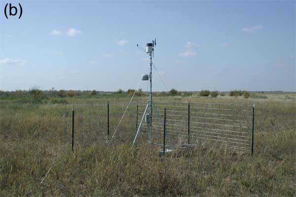
A weather station (Hobo Weather Station, Onset Computing Corp.) that measures and records a suite of meteorological data (air temperature, precipitation, relative humidity, solar radiation, and wind speed and direction) was installed on high ground in the northern portion of Plot 3 (Figures 2 and 12) on October 19, 2004. On June 2, 2005, a barometer was added to the weather station. Data are collected at 15-minute intervals and are the ending values (air temperature, relative humidity, solar radiation, and barometric pressure), averages (wind speed and direction), or summation (precipitation) for that 15-minute interval.
Figure 12--Weather station at Ashland viewed from the south (a) and east (b). Tipping-bucket rain gage is on the right end of cross bar in photograph (a), while wind-speed and direction sensors are on left end of same cross bar. Solar radiation sensor (pyranometer) is on slanted arm extending outward to the south (left) near top of weather station in photograph (b). Relative humidity and temperature sensors are in radiation shield at an elevation of two meters above lsf. Barometer is inside datalogger housing located on main pole below point where support legs connect to main pole. Dave Arnold home is in the distance in the center right of photograph (a).
Prior to installation at the Ashland site, the weather station was set up adjacent to an existing weather station at the Larned Research Site from 9/24/04 to 10/18/04 in order to assess the new station and its sensors. That assessment indicated that all sensors were operating well (i.e. sensor readings compared favorably with the readings from existing sensors at the Larned station). After installation at the Ashland site, the tipping-bucket precipitation gauge has periodically been checked through comparisons with a National Weather Service standpipe precipitation gauge mounted on the fence in the front yard of Dave Arnold's home approximately a mile north of the station (Figure 12a). Another standpipe precipitation gauge was obtained from the National Weather Service at the end of this reporting period for mounting adjacent to the weather station. In the last month of the reporting period, a hand-held unit for measuring air temperature, relative humidity, wind speed, and atmospheric pressure (Kestrel 3500 Pocket Weather Meter, Nielsen Kellerman Inc.) was obtained so that sensor operation could be checked during each site visit by the research team. Previous work at the Larned Research Site had found that the relative humidity sensor is the most likely sensor to malfunction. An additional relative humidity sensor was therefore purchased. This new sensor was configured so that it could be periodically brought to the station and left for a few weeks to check the operation of the station's relative humidity sensor. As of the end of this reporting period, all meteorological sensors appear to be operating well.
In order to enable timely assessments of weather conditions at the Ashland site, a radio modem (Onset Computing Corp.) was added to the weather station in the final weeks of the reporting period. This modem and an accompanying base station in Dave Arnold's home will allow the weather station to be programmed to send meteorological data via email at a user-defined interval. These data will also be sent to the National Weather Service in Dodge City to fill their data gap in this portion of Clark County.
The second four tasks listed in the scope of work outlined in the KWO contract involved the management, processing, and analysis of the pressure-sensor, weather-station, and neutron-probe data. Those tasks, all of which are ongoing and will continue through the life of the project, are as follows:
Each of these tasks is described in this section.
The eight sensors (five absolute-pressure miniTrolls, one Troll 9000, and two baroTrolls) used for water-level monitoring are downloaded each time the research team visits the site. Those visits are approximately every two weeks during the growing season and once every month or two at other times. Downloading is done using a hand-held (Rugged Reader, In-Situ Inc.) or laptop computer. Cables and software for downloading the sensors have also been provided to Dave Arnold and he has helped download during the winter. Each time the sensors are downloaded, the status of the internal batteries and internal memory are checked. Low (<30% capacity) batteries are changed. If the amount of occupied memory appears to be significantly increasing download time, the memory is cleared. Each time the memory is cleared, the sensor is reprogrammed and the monitoring program is restarted. A member of the research team must confirm that the monitoring program has actually restarted prior to departure from the site. When the research team downloads a sensor, a depth-to-water measurement is also taken with an electric tape (Model 101, Solinst Canada Ltd.). The same electric tape was used for all the depth-to-water measurements taken in this reporting period.
The weather station is also downloaded each time the research team visits the site. The downloading is done using a standard laptop computer. Dave Arnold also helps download the weather station during the winter. As described in the previous section, a radio modem has been attached to the weather station (not shown in Figure 12) and an accompanying base station has been set up in Dave Arnold's home to allow the weather station to be downloaded at a preset interval and the data sent via email to the KGS. The final steps in that procedure were being worked out at the close of this reporting period.
Pressure-sensor data
After downloading, the pressure-sensor data are forwarded to Dr. Xiaoyong Zhan at the KGS for processing. Dr. Zhan removes the atmospheric-pressure component from the pressure sensors submerged in the water column and adds the new data to the existing master file. The data are currently stored in Excel worksheets, but efforts have begun towards moving the data into an Oracle database. That work, however, was not completed prior to the end of this reporting period.
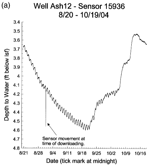
As of the completion of this report, all pressure-sensor data had been processed through the June 16, 2005, download. Because the salt-cedar control measures have yet to be fully implemented, this report does not include an in-depth analysis of the collected data. That analysis will be provided in a subsequent project report. Data from well Ash12 will be presented here to illustrate the temporal pattern of water-table variations observed at the site and to discuss two problems faced in this first reporting period.
Figures 13 and 14a-b are plots of depth to water recorded at well Ash12 for the entire reporting period, the first 60 days, and the last 60 days, respectively. The water table at well Ash12 varied over a 2.6-ft interval during the reporting period. At the start of the period in late August of 2004, plant-induced fluctuations in the water table were clearly observed (Figures 13 and 14a), as they were at well Ash22 (Figure 3a) and all other wells except well Ash32 (Figure 3b). These fluctuations die-out by mid-October as the salt cedar transition into dormancy and only reappear in May of 2005. Figures 13 and 14b illustrate the two problems that were encountered during the monitoring period. These problems, barometer submergence and incorrect temperature compensation of barometer measurements, are described in the following paragraphs.
Figure 13--Depth to water from land surface recorded in well Ash12 for the entire reporting period (well Ash12 in unaltered area [Plot 1], Figure 6a is a photograph of well and surrounding vegetation). Note high-frequency noise during winter months caused by incorrect temperature compensation of barometer readings.
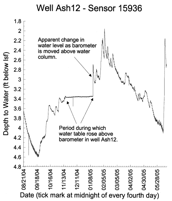
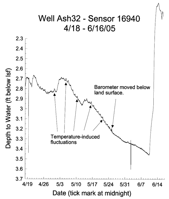
Barometer submergence--The barometers were originally placed about 5 ft below the top of casing at wells Ash12 (3.35 ft below land surface) and Ash32. Unfortunately, the water table rose more than we anticipated. At 18:45 on 11/16/04, it rose above the sensing port for the barometer (sensor 16977) in well Ash12. The submergence of that barometer is easily recognized after processing the sensor in the water column at Ash12 (sensor 15936) because all pressure changes after submergence are the same for the original sensor in the water column and the now-submerged barometer. This situation creates a horizontal line on the water-level plot for well Ash12 (Figure 13). Note that the same problem occurred at well Ash32 on 19:30 on 10/13/04 but was not recognized due to the back-up status of that barometer. Because of a delay in processing the data downloaded on December 2, we did not recognize the problem until early January 2005. A KGS staff member went to the site and raised the barometers in both wells into the surface casing (barometers in both wells raised until sensing port was 0.08 ft above lsf) on 1/13/05. This was a foot higher than had been requested and led to a new problem discussed below. Although the submergence problem is now solved, there is no way of correcting the data between 11/16/04 and 1/13/05. Fortunately, the missing water-level data are of little importance to this project because there was essentially no transpiration during this period. Barometer submergence is now checked during each site visit and an additional back-up barometer has been added to the weather station.
Figure 14--Depth to water recorded in well Ash12 for the first (a) and final (b) 60 days of the reporting period (downward spikes in water-level data [a] are commonly observed at the time of downloading because the sensor is often moved up slightly to facilitate attachment of download cable; note vertical extent of y-axis in both plots is same as in Figure 3a-b).
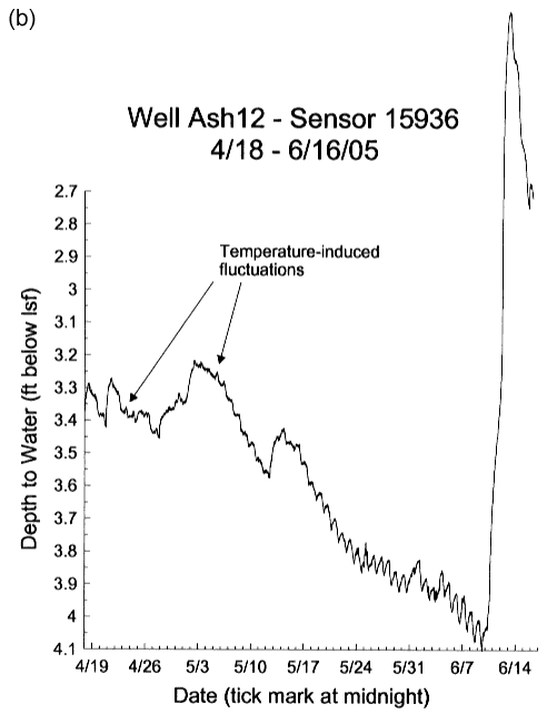
Incorrect temperature compensation of barometer measurements--The repositioning of the barometers into the surface casing resulted in a new problem. As soon as the barometers were moved up, we saw additional noise in the data (Figures 13, 14b, and 15). We attributed that noise to incorrect temperature compensation of the barometric-pressure measurement. A temperature sensor inside the barometer body provides the reading used for the temperature compensation of the pressure measurement. We attribute the noise to the time required for that temperature sensor to equilibrate with the air temperature in the casing. Prior to equilibration, the barometric-pressure measurement is not thermally compensated in the appropriate manner, producing noise in the data record. The noise characteristically is observed as an abrupt upward spike coinciding with the onset of solar heating in the morning. The spike gradually decays during the day and virtually always disappears before midnight. This problem was resolved on May 25, 2005, when Dave Arnold, at our request, lowered the barometer in well Ash12 until its sensing port was at a position 1.59 ft below land surface. The temperature-induced fluctuations abruptly ceased at that time as shown by the pressure-sensor data from well Ash32 (Figure 15). On June 2, 2005, we moved the back-up barometer in well Ash32 to a sensing-port position of 1.56 ft below lsf. We are currently working on procedures to remove the noise produced by incorrect temperature compensation from the data. Our current procedure exploits the fact that water levels at Ash32 are not subject to the variations induced by plant-water use as at the other wells and therefore display a very smooth variation through time (Figures 3b and 15).
Figure 15--Depth to water recorded in well Ash32 for the final 60 days of the reporting period (note downward spikes in water-level data at time of downloading as in Figure 14a; barometer [sensor 16977] moved 1.59 ft below lsf on May 25, 2005).
Weather-station data
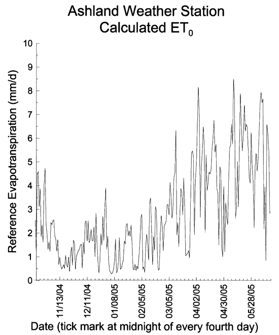
After downloading, the weather-station data are forwarded to Dr. Zhan for processing. Dr. Zhan adds the new data to the existing master file and calculates the reference evapotranspiration parameter (ET0--Allen et al. [1998]) based on the Penman-Monteith equation [Campbell and Norman, 1998] to characterize the potential for evapotranspiration when water is not a limiting factor. The data are currently stored in Excel worksheets, but efforts have begun to move the data into an Oracle database that will be accessible on the Internet. That work, however, was not completed prior to the end of this reporting period.
Figure 16 displays the reference evapotranspiration parameter for the entire period during which the weather station was operating. The decrease in ET0 in the winter months and the increase in the spring are as expected. The sizable temporal variations in ET0 observed throughout the period also are as expected and are a product of changing meteorological conditions.
Figure 16--Calculated reference ET0 for entire duration of weather station operation during this reporting period.
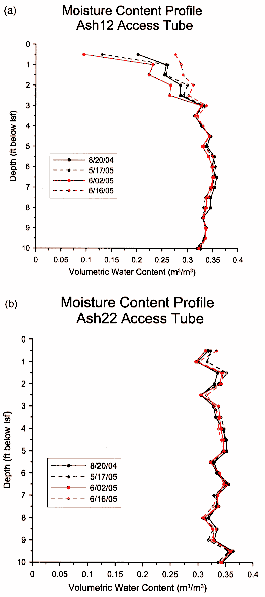
Measurements of moisture content in the access tubes adjacent to each well were recorded with a neutron probe (Model 503 DR Hydroprobe Moisture Depth Gauge; Campbell Pacific Nuclear) using a count duration of 16 s and depth increments of 0.5 ft. Standard counts were recorded in the field both prior to and after access tube measurements. Note that this contract provided support for installation of the neutron-probe access tubes but not for travel to the Ashland site to perform the logging. Thus, only one set of logs (obtained on August 20, 2004 at the time of installation) was obtained in the August 2004 to April 2005 period. After that time, the research team obtained funding from the Kansas Water Resources Institute to support travel to the site to perform the neutron logging.
The neutron logging data were processed at KSU. The mean standard count for the duration of the study was used to convert each measured count to a count ratio (CR). The soil volumetric water content (m3 m-3), Θ, corresponding to each measured count ratio was calculated with the calibration equation Θ = 0.2929 x CR - 0.0117, which was based on laboratory calibrations and an adjustment for PVC pipe. However, the calculated moisture content values are subject to revision because of the sensitivity of the neutron probe results to soil salinity. As shown by the direct-push EC logs presented earlier, the Ashland soils have very high EC readings, which may affect the results of the neutron logging.
Figures 17a-b display results of neutron logging at access tubes adjacent to wells Ash12 and Ash22, respectively. The large differences between the moisture content profiles from the Ash12 access tube, particularly in the first foot, are undoubtedly due to the existence of coarse (i.e. rapidly drained) material near the surface (see low EC values near surface in log of Figure 6b). The small differences observed between the moisture content profiles from the Ash22 access tube are consistent with the high EC values (suspected clayey soil zone) observed near the surface at that well (see Figure 8b). These readings may be influenced by salinity as indicated in the previous paragraph. However, the total porosity values below the water table appear reasonable for both access tubes.
Figure 17--Volumetric water content versus depth plot from neutron-probe access tube adjacent to well Ash12 (a) and well Ash22 (b).
(work cited in text, project presentations (*), or general references (**))
Allen, R.G., Pereira, L.S., Raes, D., and Smith, M., 1998, Crop evapotranspiration--Guidelines for computing crop water requirements: Food and Agricultural Organization of the United Nations, Rome, FAO Irrigation and Drainage Paper 56.
Butler, J.J., Jr., Healey, J.M., Zheng, L., McCall, W., and Schulmeister, M.K., 1999, Hydrostratigraphic characterization of unconsolidated alluvial deposits with direct-push sensor technology: Kansas Geological Survey, Open-File Report 99-40, 30 pp. [Available online]
*Butler, J.J., Jr., Kluitenberg, G.J., Whittemore, D.O., Healey, J.M., and Zhan, X., 2005, Quantifying ground-water savings achieved by salt-cedar control measures: A demonstration project: Eos Trans. AGU, v. 86, no. 18, Jt. Assem. Suppl., Abstract H33B-06. (poster presented at a special session entitled "Measurement and Monitoring Methods in Ecohydrology" at the Spring Meeting of the American Geophysical Union, New Orleans, May 25, 2005). [Available online]
*Butler, J.J., Jr., Kluitenberg, G.J., and Whittemore, D.O., 2004, Assessment of changes in ground water availability associated with a salt cedar control project in Clark County: presentation at a salt-cedar control workshop hosted by the Kansas Alliance for Wetlands and Streams and the Kansas Grazing Lands Coalition, Ashland, October 6, 2004.
Butler, J.J., Jr., Kluitenberg, G.J., Whittemore, D.O., Loheide, S.P., II, Jin, W., Billinger, M., and Zhan, X., in review, A field investigation of phreatophyte-induced fluctuations in the water table, manuscript under review by coauthors.
Campbell, G.S., and Norman, J.M., 1998, An Introduction to Environmental Biophysics: Springer, New York, 286 pp.
**Glenn, E.P., and Nagler, P.L., 2005, Comparative ecophysiology of Tamarix ramosissima and native trees in western U.S. riparian zones: Jour. of Arid Environments, in press.
**Shafroth, P.B., Cleverly, J.R., Dudley, T.L., Taylor, J.P., Van Riper, C., III, Weeks, E.P., and Stuart, J.N.,, 2005, Control of Tamarix in the western United States: Implications for water salvage, wildlife use, and riparian restoration: Environmental Management 35(3), 231-246.
Schulmeister, M.K., Butler, J.J., Jr., Healey, J.M., Zheng, L., Wysocki, D.A., and McCall, G.W., 2003, Direct-push electrical conductivity logging for high-resolution hydrostratigraphic characterization: Ground Water Monit. and Remed. 23(3), 52-62.
Kansas Geological Survey, Geohydrology
Placed online Feb. 1, 2006
Comments to webadmin@kgs.ku.edu
The URL for this page is http://www.kgs.ku.edu/Hydro/Publications/2005/OFR05_19/index.html