Kansas Geological Survey, Open-file Report 94-28e
Part of the Mineral Intrusion Project: Investigation of Salt Contamination of Ground Water in the Eastern Great Bend Prairie Aquifer
A cooperative investigation by The Kansas Geological Survey and Big Bend Groundwater Management District No. 5
KGS Open File Report 94-28e
Released December, 1994
To read this report, you will need the Acrobat PDF Reader, available free from Adobe.
Substantial effort has gone into developing an understanding of the amount of salt at each monitoring well site, the details of its distribution, the rates and patterns of change over time, and the hydrogeologic features that control these processes (OFR 94-28b-d). Although more data are needed, we have now reached a point where we can carry out some initial analysis of system-level characteristics and behavior. These results will have implications for the conceptual and numerical models under development, and will guide future measurements and calculations.
Budgetary analysis is a somewhat imprecise but very powerful tool for analysis of natural systems. Figure E1 illustrates its application in our particular case. We can identify a box representing some specific volume of the aquifer. It may be the volume around an individual well, or the total volume beneath a section, a township, or some larger region. That volume will contain a certain amount of water, and a certain amount of salt--both of which might be relatively constant or might vary over time.
Figure E1--An illustration of the water and salt budget process. Conservation of mass requires that any difference between inflow and outflow must be reflected by a change in inventory. If the inventory is constant the fluxes are in balance and the system is said to be in "steady state".
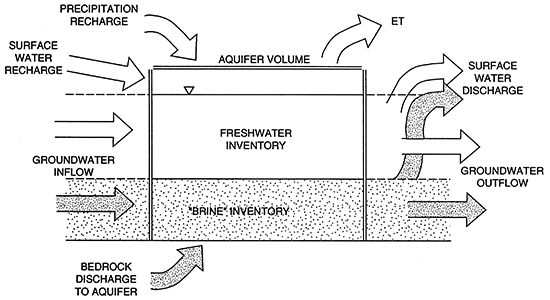
However, the total masses of both water and salt must be conserved; the change in volume (or inventory) within the box must be equal to the difference between the amount that comes in and the amount that goes out (this is exactly the same process used in the much more rigorous mathematical approach discussed in the report on modeling, OFR 94-28f). If the inventory is nearly constant, then inflow must equal outflow, and this equilibrium (or more accurately, quasi-equilibrium) condition is commonly referred to as "steady-state." If the relative proportions of the fresh water and the salt remain constant, then the same must be true, on average, for the ratios of freshwater inflow to salt inflow, and of freshwater outflow to salt outflow.
This simple set of conclusions provides a great deal of leverage for interpreting the situation. Salt may enter the box by upward flow from the bedrock or by lateral flow within the aquifer; it can leave by lateral groundwater flow or by discharge to outflowing surface water (in principle it can also leave by re-entry into the bedrock, but this pathway will be neglected initially). Freshwater can enter by all the same pathways, and also from recharge of both surface inflow and precipitation. It has the same outflow pathways as salt, with the addition of evapotranspiration.
Some of these budgetary terms are more easily measured or estimated than others. They have different characteristics of variability; for example, we may not know the groundwater inflow term with high accuracy, but because aquifer permeabilities do not change and head gradients vary only slightly, we know that the term is relatively constant. By comparison, we can measure streamflow or precipitation at a given point with high accuracy, but they are extremely variable in time and space. Because of this situation, the additional information that budget terms must add up to a certain value or remain in a fixed ratio to certain other terms is extremely important. The budgetary approach adds several equations to the assembly of unknown quantities that we are trying to decipher, and permits us to evaluate possible mechanisms. Budgetary failure -- that is, when things "don't add up" -- are particularly helpful, since they let us know that we need to re-examine either our data or our hypotheses.
Table E1 presents data for both 1993 and 1994 on the chloride mass (mg) per square foot of the aquifer surface for each of the sites where an inventory could be constructed by the methods described in OFR 94-28b. Sites 50-52 are included to show the calculated values from sites that do not have wells penetrating the Permian; all three overlie Cretaceous bedrock. Of the sites that overlie Cretaceous bedrock (4, 6, 7, 50, 51, and 52), only site 4 was found to have appreciable salinity at the base of the aquifer.
Table E1a--Salt Inventory at monitoring well sites in the Minerai Intrusion study area (1993).
| Site.well no. | Depth to Bedrock |
Depth to Water Table |
Area Under Chloride Profile |
Chloride Mass per Unit Area |
Equivalent 42k Concen. Sat. Thick |
|---|---|---|---|---|---|
| 1.1 | 146 | 5.3 | 6.43E+05 | 2.91E+06 | 15.308 |
| SP | 186 | 10.8 | 7.96E+05 | 3.60E+06 | 18.94 |
| 3.1 | 130 | 25.73 | 33561 | 1.52E+05 | 0.79907 |
| 4.1 | 129 | 8.7 | 1.91E+05 | 8.66E+05 | 4.5492 |
| 5.1 | 181 | 1.77 | 3.06E+06 | 1.39E+07 | 72.775 |
| 8.1 | 118.3(1) | 8.8 | 68715 | 3.11E+05 | 1.6361 |
| 9.1 | 87 | 9 | 1.96E+05 | 8.89E+05 | 4.6693 |
| 10.1 | 156 | 18.3 | 84985 | 3.85E+05 | 2.0234 |
| 11.1 | 208 | 13.5 | 8.65E+05 | 3.92E+06 | 20.592 |
| 16.1 | 220 | 11.98 | 1.68E+06 | 7.60E+06 | 39.915 |
| 17.1 | 114 | 11.6 | 2.49E+05 | 1.13E+06 | 5.9393 |
| 18.1 | 214 | 19.25 | 8.52E+05 | 3.86E+06 | 20.295 |
| 21.1 | 137 | 21.6 | 2.67E+05 | 1.21E+06 | 6.3524 |
| 22.1 | 215 | 16.1 | 8.07E+05 | 3.66E+06 | 19.208 |
| 23.1 | 94 | 21.42 | 41453 | 1.88E+05 | 0.98698 |
| 24.1 | 123 | 21 | 3.65E+05 | 1.66E+06 | 8.6993 |
| 25.1 | 98 | 6.3 | 1.31E+06 | 5.95E+06 | 31.241 |
| 26.1 | 177 | 6.8 | 9.52E+05 | 4.31E+06 | 22.661 |
| 27.1 | 104 | 10.12 | 82905 | 3. 76E+05 | 1.9739 |
| 30.1 | 138 | 14.54 | 56876 | 2.58E+05 | 1.3542 |
| 31.1 | 93 | 13.65 | 37273 | 1.69E+05 | 0.88746 |
| 32.1 | 172 | 2.6 | 2.48E+05 | 1.12E+06 | 5.9067 |
| 36.1 | 195 | 28 | 4. 26E+05 | 1.93E+06 | 10.15 |
| 37.1 | 240 | 58.63 | 95705 | 4. 34E+05 | 2.2787 |
| 42.1 | 160 | 13.03 | 1.53E+05 | 6.91E+05 | 3.6311 |
| 43.1 | 65 | 4.87 | 71699 | 3.25E+05 | 1.7071 |
| 50.1 | 223 | 26.15 | 13657 | 61885 | 0.32518 |
| 51.1 | 200 | 17.3 | 23314 | 1.06E+05 | 0.5551 |
| 52.1 | 221 | 30.79 | 15816 | 71667 | 0.37658 |
| Notes: (1) Depth to bedrock changed from 117 ft based on inspection of conductivity log. Depths and thicknesses in feet; Area = (mg-ft)/L; mass = (mg/sq. ft). |
|||||
Table E1b--Salt Inventory at monitoring well sites in the Mineral Intrusion study area (1994).
| Site.well no. | Depth to Bedrock |
Depth to Water Table |
Area Under Chloride Profile |
Chloride Mass per Unit Area |
Equivalent 42k Concen. Sat. Thick |
|---|---|---|---|---|---|
| 1.1 | 146 | 6.35 | 6.10E+05 | 2.76E+06 | 14.517 |
| SP | 186 | 11.3 | 8.05E+05 | 3.65E+06 | 19.172 |
| 3.1 | 130 | 20.54 | 32818 | 1.49E+05 | 0.78138 |
| 4.1 | 129 | 7.87 | 2.17E+05 | 9.82E+05 | 5.1603 |
| 5.1 | 181 | 2.08 | 3.05E+06 | 1.38E+07 | 72.522 |
| 8.1 | 118.3(1) | 11.1 | 75413 | 3.42E+05 | 1.7955 |
| 9.1 | 87 | 9.36 | 2.07E+05 | 9.39E+05 | 4.9332 |
| 10.1 | 156 | 13.75 | 79998 | 3.62E+05 | 1.9047 |
| 11.1 | 208 | 11.39 | 8.04E+05 | 3.64E+06 | 19.135 |
| 16.1 | 220 | 7.64 | 1.66E+06 | 7.50E+06 | 39.412 |
| 17.1 | 114 | 10.54 | 2.57E+05 | 1.16E+06 | 6.1104 |
| 18.1 | 214 | 11.02 | 8.59E+05 | 3.89E+06 | 20.454 |
| 21.1 | 137 | 23.07 | 2.16E+05 | 9.80E+05 | 5.1505 |
| 22.1 | 215 | 12.71 | 8.09E+05 | 3.67E+06 | 19.267 |
| 23.1 | 94 | 22.4 | 40763 | 1.85E+05 | 0.97055 |
| 24.1 | 123 | 23.9 | 2.57E+05 | 1.16E+06 | 6.1079 |
| 25.1 | 98 | 6.02 | 1.32E+06 | 6.00E+06 | 31.535 |
| 26.1 | 177 | 8.76 | 1.03E+06 | 4.66E+06 | 24.47 |
| 27.1 | 104 | 11.22 | 1.09E+05 | 4.92E+05 | 2.5833 |
| 30.1 | 138 | 17.19 | 47496 | 2. 15E+05 | 1.1308 |
| 31.1 | 93 | 15.06 | 35320 | 1.60E+05 | 0.84096 |
| 32.1 | 172 | 9.1 | 2.60E+05 | 1.18E+06 | 6.1963 |
| 36.1 | 195 | 27.84 | 4.30E+05 | 1.95E+06 | 10.249 |
| 37.1 | 240 | 57.1 | 92821 | 4.21E+05 | 2.21 |
| 42.1 | 160 | 13.01 | 1.50E+05 | 6.79E+05 | 3.5671 |
| 43.1 | 65 | 5.14 | 81034 | 3.67E+05 | 1.9294 |
| 49.1 | 106 | 1 | 196670 | 8.91E+05 | 4.6826 |
| 50.1 | 223 | 22.34 | 14846 | 67271 | 0.35348 |
| 51.1 | 200 | 13.68 | 24149 | 1.09E+05 | 0.57498 |
| 52.1 | 221 | 23.67 | 16859 | 76390 | 0.40139 |
| Notes: (1) Depth to bedrock changed from 117 ft based on inspection of conductivity log. Depths and thicknesses in feet; Area = (mg-ft)/L; mass = (mg/sq. ft). |
|||||
Table E1 shows that site 5 has by far (an order of magnitude) more salt within the aquifer compared to the other sites. Because site 5 required extrapolation of the deepest, saltiest portion of the chloride concentration profile to bedrock (-30 ft worth; methods explained in OFR 94-28b), the mass is influenced by the fitted-curve transition zone using a maximum of 42,000 mg/L. If the fitted curve is recalculated to a maximum of 32,000 mg/L (the approximate maximum concentration at the bottom of the actual logged profile), the mass is only reduced by about 10%--still an order of magnitude greater than any other site. Site 5 is apparently atypical, compared to the other sites, in that it is located directly upon the Permian Cedar Hills Sandstone subcrop and is close to Rattlesnake Creek, a gaining stream. This location is probably responsible for the unusually thick and massive salt-water profile presented by site 5.
Also shown in Table E1 is the equivalent saturated thickness of typical Permian brine to which this amount of chloride would correspond. This latter value is based on estimates (D. O. Whittemore, pers. comm.) of typical concentration levels for the two end members of the groundwater mixing process. For the Stafford County area, native brine is taken as having a specific conductance of 100,000 µS/cm (or 10,000 mS/m), total dissolved solids (TDS) of 75,000 mg/L, and a chloride concentration of 42,000 mg/L. Uncontaminated fresh water in the upper part of the Great Bend Prairie aquifer is taken as having specific conductance equal to 400 µS/cm (or 40 mS/m), TDS = 250 mg/L, and chloride = 10 mg/L.
Using the equivalent volume of a concentrated source brine instead of the actual salt inventory (in mass of salt per unit area of aquifer surface) makes it much easier to visualize comparisons of salt and water, and it relates the salt back to some ultimate source. We have to be careful not to overuse this budgetary convenience, however, since we know that the actual concentrations of salt in the bedrock pore water are much less than the theoretical brine value in many areas.
The remainder of the discussion will focus primarily on the northern part of the study area; work on the less saline southern part is in progress and will be presented later. Figure E2 is a map of the northern region, showing relative inventories of brine and fresh water and the extent of the mixing between the two (indicated by the 500 mg/L chloride value). These values are scaled to the numerical values in Table E1. The addition of the zone of mixed salt- and freshwater is of little use from a budgetary standpoint because of concentration variations within the mixed zone, but it is of great practical importance. Waters with 3,000 mg/L chloride and with 10,000 mg/L are very different from a salt budget viewpoint, but are essentially the same from a water quality standpoint--unusable for most purposes. Further, the extent of mixing gives us valuable process information about the extent of vertical water movement within the aquifer and about the horizontal coupling between "boxes."
Figure E2--A representation of the total saturated thickness (height of column) and the saturated thickness that would be occupied by the volume of Permian brine equivalent to the salt content of the total water column (height of dark column). At each site, 1993 values are on the left, 1994 on the right. The height of 500 mg/L limit of the mixed zone is shown by light stippling; this has no budgetary significance, but shows the extent of vertical mixing and the amount of usable fresh water at each site.
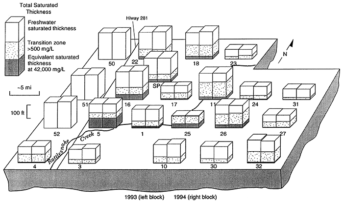
The data in Table E1 and Figure E2 demonstrate some things that are well known; for example, the very thick transition zone and the near absence of usable fresh water in the vicinity of the Quivira marshes (see also Figures C9 and C10, OFR 94-28c). However, it also shows that the actual equivalent brine inventories are higher in the western part of the study area than in the east. This same observation holds in the less saline southern part of the study area, where the highest equivalent brine concentrations are at sites 36, 37, 42 and 43 (see site maps, OFR 94-28 a and c). This geographic association does not prove, but tends to support, the idea that the subcrop of the Cedar Hills Sandstone (see Fig. A2, OFR 94-28a) may be a larger source of brine discharge than the other Permian formations farther to the east. Further implications of the inventory variations will be discussed below.
The first point to consider is whether we can legitimately apply steady-state assumptions to the system. The data in OFR 94-28b indicate clearly that there has been less than a one percent variation in salt inventories between 1993 and 1994, and the concentration elevations discussed in OFR 94-28c confirm the stability of the system on this time scale. Head and salt concentration (Whittemore, 1993) measurements over the approximately l5-year period since the monitoring well network was installed suggest that there have not been major changes in the system on this time scale. Overall, we can reasonably treat the salt content as being in steady-state as a first approximation.
Freshwater inventories are somewhat more variable on a short time scale. However, 1993 was a year of unusually high (perhaps record) recharge, so we can compare this change with the inventory. Figure C2 in OFR 94-28c shows that the northern monitoring well sites experienced water table recharge ranging from one to eleven feet in 1993. Even after allowance for saltwater in the saturated thickness, most of these sites have a freshwater inventory (total saturated thickness minus equivalent brine thickness) equivalent to a saturated thickness of 100 ft or more, so changes of several feet are only a few percent of the freshwater inventory--and that in an extreme year. On the longer term, we know that present water levels in the area are within 10 ft or so of estimated predevelopment levels (Mitchell et al., 1994). To a good first approximation we may therefore also treat the freshwater inventory as being in steady state.
Young (1992, figures 9 and 10) presented maps of the potentiometric surfaces of both the Great Bend Prairie aquifer and the Cedar Hills Sandstone formation. These indicate that groundwater flow in both the Quaternary and Permian aquifers is to the east or east-northeast in the area of interest. This means that the west-to-east decrease in salt inventory requires explanation. Although averaging a spatially variable quantity such as salt inventory is not a precise approach, we can make some sub-regional estimates by considering the five "saltwater" townships for which we have at inventory data at least on the township corners. These are T21S, R11-12W and T22S, R10-12W. Table E2 presents average inventory data in terms of saturated thickness of equivalent brine, based on the data in Table E1 for 1994. Because we are comparing units of the same surface area, the height of the brine-saturated thickness is directly proportional to the volume of brine and the mass of salt.
Table E2--Estimated 1994 Salt Inventory (Average Equivalent Brine Saturation).
| Township | Sat (ft) | Brine (ft) | % Brine | Sites |
|---|---|---|---|---|
| 21S12W | 179 | 20.9 | 12 | 22, 16, 17, 18, SP |
| 21S11W | 144 | 11.7 | 8 | 18, 17,23,11 |
| 22S12W | 159 | 33.1 | 21 | 16, 5, 17, 1 |
| 22S11W | 133 | 17.8 | 13 | 17, 1, 11, 25 |
| 22S10W | 139 | 20.3 | 15 | 11, 24, 25, 26 |
If the groundwater flow direction is basically from west to east, and groundwater flow is the primary mechanism for salt transport, we would expect the salt inventories to remain constant from west to east if the Cedar Hills is the sole source of salt discharge, and to increase from west to east if there is general salt discharge from the Permian all along the flow path. Instead, the data suggest that there may be a decrease in inventory from west to east. Some of the possible explanations for that, and their implications for future research, are:
All of the above approaches will be addressed in an effort to refine our understanding of the salt inventory and the processes that control it.
Another aspect of the budgetary approach is the estimation and comparison of discharge, recharge and groundwater flux terms in the water budget equation. A few preliminary estimates of the Permian discharge were presented in OFR 94-28d. It is worthwhile to expand on the comments there to illustrate how this approach can be applied.
Sophocleous (1992a), using optimized computer (MODFLOW) simulations, has suggested that in the lower Rattlesnake basin recharge represents about 80% of the input of fresh water on a predevelopment basis, and a similar percentage at present if changes in storage due to pumping are neglected. Most of the rest is groundwater inflow, with a minor amount due to stream-derived recharge. A summary of recharge estimates for the area shows (Sophocleous 1992b) that the long-term average recharge is probably about 2"/yr, and certainly in the range of 1-6".
If we assume steady state and consider the brine/freshwater ratios implied by Table E2, then the average brine-equivalent Permian discharge should be on the order of 10-20% of the freshwater recharge; that is, on the order of magnitude of about 0.0001 ft3/ft2/day of end-member brine. There are either head gradient, or flux data, or both available for seven sites in the northern saline region (OFR 94-28d): sites 1, 5, 16, 17, 18, 25, 27, and SP. Density corrected head data suggest that the vertical head gradient favors upward flow (discharge from the Permian) at all but site 17. Because of known problems with the wells or the permeability determinations, we do not trust the very high values of Permian discharge that could be derived from sites 1 and possibly 5; however, both have substantial salt inventories, so positive discharge values are consistent with the observations. Of the remaining five wells, the estimated fluid fluxes range from 0.001 to 0.03 ft3/ft2/day; 4 are positive (discharge) and site 17 is negative. These values are 1 to 2 orders of magnitude higher than the steady-state brine-equivalent discharge estimated from recharge rates. As above, we can consider the possible explanations:
The foregoing material both illustrates the importance of the budgetary approach, and provides a first listing of important questions and needed work. It seems likely that brine discharge occurs predominantly in the western part of the study area, with mixing occurring near discharge sites and during the course of eastward flow. Short-term data suggest an approximately steady-state inventory of salt, but both the spatial distribution and flux rate estimates hint at the possibility of disequilibrium. It will be very important to obtain a better evaluation of the budget terms, both by site-specific measurements and by refined calculations and modeling, in order to evaluate whether the present inventory really is in approximate equilibrium with the present discharge rates. Many of these efforts will be the focus of work in the coming year.
Mitchell, J. E., Woods, J., McClain, T. J., and Buddemeier, R. W., 1994. January 1993 Kansas Water Levels and Data Related to Water-Level Changes: Kansas Geological Survey, Technical Series 4, 114 pp.
Sophocleous, M. A., 1992a. Modifications and Improvements on the Lower Rattlesnake Creek-Quivira Marsh Stream-Aquifer Numerical Model: Kansas Geological Survey, Open-File Report 92-37, 15 pp.
Sophocleous, M. A., 1992b. A Quarter-Century of Ground-Water Recharge Estimates for the Great Bend Prairie Aquifer of Kansas (1967-1992): Kansas Geological Survey, Open-File Report 92-17, 22 pp.
Whittemore, D. O., 1993. Ground-water geochemistry in the mineral intrusion area of Groundwater Management District No. 5, south-central Kansas: Kansas Geological Survey, Open-File Report 93-2.
Young, D. P., 1992. Mineral Intrusion: Geohydrology of Permian Bedrock Underlying the Great Bend Prairie Aquifer in South-Central Kansas: Kansas Geological Survey, Open-file Report 92-44, 47 pp. [available online]
Kansas Geological Survey, Geohydrology
Placed online Feb. 19, 2016; originally released Dec., 1994
Comments to webadmin@kgs.ku.edu
The URL for this page is http://www.kgs.ku.edu/Hydro/Publications/1994/OFR94_28e/index.html