Kansas Geological Survey, Open-file Report 2000-6
by Jianghai Xia,
Rick Miller,
and Dana Adkins-Heljeson
Kansas Geological Survey
KGS Open-file Report 2000-6
Feb. 2, 2000
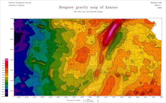
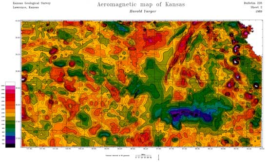
The potential-field database at the Kansas Geological Survey (KGS) contains 72,000 line-km (45,000 line-mi) of regional aeromagnetic data and 62,606 gravity-station measurements. All data are in ASCII format and stored on CD-ROM. The CD-ROM can be read by a PC with Microsoft Windows9x. This open-file report provides background information on the potential-field data acquisition and reduction. The Bouger gravity map of Kansas was published in 1992 (Xia et al., 1992) and the aeromagnetic map of Kansas was published in 1981 (Yarger et al., 1981). A series of processed and/or interpreted maps were published in 1995 (Xia et al., 1995a, 1995b, 1995c, 1995d, 1995e, 1995f). For data processing and interpretation, readers can also refer to Lam (1989), Lam and Yarger (1989), Xia (1992 and 1996), Xia and Sprowl (1995), Xia et al. (1992, 1993, 1995g, and 1996), and Yarger (1983a, 1983b, 1985, and 1989), and Yarger etal. (1978 and 1981).
The most direct use of gravity survey data in Kansas is to map underground-mass distributions. The reference gravity formula, which will be given in the next section, represents the average distribution of gravity on the whole surface of the Earth. The value of a gravity measurement at a particular point is usually not equal to the value calculated by the formula at the point. One reason for that difference is that underground-mass distributions are irregular. This difference can be used under some constraints to determine irregular mass distributions. There are large-scale problems related to the constitution of continents and oceans, or large mountain ranges and oceanic trenches. Smaller-scale problems include local geological structures; still smaller problems are those related to exploration of underground natural resources, such as oil; the smallest-scale problems are those related to environmental, engineering, and groundwater, for which the microgravity survey measurement spacing could be less than 1 m (3.3 ft).
Phanerozoic sedimentary rocks with a thickness of 170 m (560 ft) to 3,300 m (10,800 ft), cover virtually all of the Precambrian basement in Kansas, except for a large inclusion of Precambrian granite found in the Cretaceous mica peridotite of the Rose Dome in Woodson County (Bickford et al., 1971; Franks et al., 1971). The sediments were generally deposited on a near-horizontal surface resulting in a state with little lateral density change. There clearly is a density difference between the sediments and Precambrian basement. The Moho discontinuity is the main source of gravity variability.
The survey scale which we used in Kansas, a measurement spacing of about 1.6 km (1 mi) by 1.6 km (1 mi) in eastern Kansas and 1.6 km (1 mi) by 3.2 km (2 mi) in western Kansas allows us to determine the depth to the Precambrian basement, the thickness of the Earth's crust, to determine possible rock types in the upper part of the Precambrian basement, and to predict locations of interesting shallow structures.
Gravity stations in Kansas. A larger version of this figure is available.
In the earliest stage of the gravity survey in northeastern Kansas a Worden gravimeter was used with 0.01 mGal/division precision. The total number of gravity-station measurements with that meter is about 5,000. LaCoste and Romberg (L&R) model G and model D gravimeters were used to collect an additional ~57,000 gravity-station measurements.
The Worden and L&R gravimeters are relative instruments, which measure the difference in gravity between two stations. The absolute gravity value of a station is known by comparison with a reference station, which has a known absolute gravity value. The absolute gravity value at a reference station is determined by a pendulum meter or falling-body methods. The Department of Defense has established several reference stations in Kansas.
The L&R model D gravimeter has a range of 200 mGal with a reset for world wide operation, a read accuracy of plus or minus 0.005 mGal (which means the meter can tell the difference of one in two hundred millions of the normal gravity field), and a drift rate of less than 1 mGal/month. The L&R model D gravimeter is sealed to eliminate any effect from changes in the atmospheric pressure. As safety precaution, they are also internally pressure compensated. The sensor is completely demagnetized and then enclosed within a magnetic shield. The gravimeter, carrying case, and battery weight about 19 pounds.
The L&R model D gravimeter uses a zero length elastic spring suspended in a metastable equilibrium state. A zero length spring is a spring with a zero length when it does not carry a mass. A zero length spring's restoring force is proportional to the total length of the spring. Gravity change is linearly related to the length change of the zero length spring. The meter measures the length change of the spring (![]() L) between two stations, the gravity change can be known by simply multiplying
L) between two stations, the gravity change can be known by simply multiplying ![]() L with a meter calibration factor c. The meter calibration factor is determined by taking repeated readings at two gravity stations with a known gravity change (
L with a meter calibration factor c. The meter calibration factor is determined by taking repeated readings at two gravity stations with a known gravity change (![]() g), i.e., c =
g), i.e., c =![]() g/
g/![]() R, where
R, where ![]() R is the average change in reading between these two stations. The calibration factors of the L&R model D meters used in the Kansas survey are about 1.0 to convert readings to mGal units.
R is the average change in reading between these two stations. The calibration factors of the L&R model D meters used in the Kansas survey are about 1.0 to convert readings to mGal units.
The area of the state of Kansas was divided into a number of rectangular blocks. Each of the blocks has dimensions of approximately 40 km (25 mi) in the east-west direction and 26 km (16 mi) in the north-south direction. This gravity survey was completed block by block. A KGS base station was chosen and located about the center of each block. A KGS base station is a station which supports all field stations within the block. Field stations are gravity measurement points in the field and the absolute gravity value of field stations are derived from the KGS base station. KGS base stations were also used to monitor the meter drift. A KGS base station was occupied three to five times a day, with three to four hours separating successive readings. The first meter reading must be taken at the beginning of the work day and the last meter reading at the end of the work day must be completed at the base station.
The absolute gravity value of the KGS base stations were determined by connecting them to a nearby Department of Defense (DOD) station, which was referenced to the International Gravity Standardization Net 1971 (IGSN71) (Morelli et al., 1974). The IGSN71 is a world-wide net of reference gravity stations with established absolute gravity values. A subset of the DOD base stations belong to the IGSN71, with the rest being an extension of the net covering the United States. The average accuracy of the DOD base stations used in the gravity survey in Kansas is 0.1 mGal (Lam, 1986). The KGS base stations were an extension of the DOD base station net. The absolute gravity value of the KGS base stations were calculated by repeating readings at a DOD station and a KGS base station, a reading loop was D--B--D--B--D (start taking the first reading at a DOD station, ahead to a KGS base station to take the second reading, looping back to the DOD for the third reading, then on to the KGS base station to take the fourth reading, and the last reading was ended at the DOD station) or B--D--B--D--B. The average difference between the DOD station and the KGS base station was calculated by the five readings. The absolute value of the KGS base station was equal to the absolute gravity value of the DOD station plus the average difference.
The accuracy of the KGS base stations was controlled by readings on overlap stations. Stations along the eastern and western boundaries of each block were occupied twice. These were called overlap stations. This 4% redundancy allowed for error checking and quality control. The differences in overlap readings were used to adjust the absolute gravity value of the KGS base stations so that the differences in overlap readings were minimized after modifying the absolute gravity value of the KGS base stations. The double readings at overlap stations allowed us to estimate accuracy of the gravity readings, which was 0.064 mGal of the rms error (Xia, 1992).
Gravity stations were normally located at the comer of a 1.6 km (1 mi) section, usually at a road intersection or a fence line. When a particular section comer was not accessible by vehicles, a replacement point nearby was taken instead. The measurements were taken every 1.6 km (1 mi) along parallel east-west roads spaced 3.2 km (2 mi) apart in western Kansas (west of longitude 98.30°) and every 1.6 km (1 mi) along parallel east-west roads spaced 1.6 km (1 mi) apart in eastern Kansas. Measurements extend slightly into the surrounding states. The total number of gravity-station measurements is 62,606.
United States Geological Survey (USGS) 7.5 minute topographic maps were used in navigation and determining the station elevation. These maps cover an area 7.5 minutes longitude by 7.5 minutes latitude, i.e., 11 by 13.5 km or 7 by 8.5 mi. Roads, landmarks, and section lines are also shown on these maps. They are normally contoured at 10 feet elevation intervals (accurate to the nearest foot) labeled at section corners, midway between two adjacent section corners, as well as on benchmarks. Once in a while, elevation was not labeled on the map at a gravity station. In that case the elevation was estimated by interpolating between contour lines (Lam, 1986).
In practice, a gravity crew may not exactly locate the meter at the point which is shown on the maps. The rms error in north-south location is definitely less than 10 m (33 ft) because width of county roads are usually less than 20 m (66 ft), so that the rms error associated with the horizontal location would be less than 0.013 mGal. The elevation of gravity station was taken within an accuracy of 0.3 m (1 ft), so that the rms error associated with elevation would be less than 0.059 mGal. The overall accuracy of the Bouguer gravity data in Kansas is 0.150-0.200 mGal if the errors in DOD stations are not taken into account (Xia, 1992).
There are two kinds of corrections that must be applied to raw field data. One is related to time. If a gravity meter is at a station and not moved, readings taken from the meter will change with time. There are two main causes for the changes. One is the nominal drift of the meter (the spring and the associated mountings and connections are not perfectly stable, and slow or abrupt changes may occur). In addition to the drift from internal causes there are external variations of gravity which result from the variation in the gravitational attraction of the Sun and Moon (the Earth tide) as well as the resulting deformation of the Earth (the solid Earth tide) as their positions change with respect to the Earth. They have a maximum amplitude of about 0.3 mGal and occur in a period as short as about 6 hours.
The other kind of corrections are related to space, and normally include the latitude correction, the free-air correction, the Bouguer correction, and the terrain correction.
To provide data for the drift and tide corrections, the gravity meter is returned to a base station at intervals determined based on the stability of the meter and the precision expected for the survey. In the survey of Kansas, the meters are returned to base stations at less than 4-hour intervals. The difference in the two successive readings at the same base station is the combination of the tidal and drift effects and should be eliminated by the tidal and drift corrections.
Theoretical tidal gravity effects can be calculated for any time and location. An expression for the tidal gravity effects could be found in Longman (1959). After taking out the tidal effects from the difference in the two successive readings at the same base station, the remainder is used to determine the drift rate (in mGal/minute) between the two successive base readings. This rate is used to calculate drift from the reading time at each intermediate station. For example, the first base reading is 980,638.010 mGal (after multiplying a meter calibration factor and knowing the absolute gravity value at the base station) at 10:30 am and the second base reading is 980,638.025 mGal at 12:10 p.m., so that the difference in the two successive base readings is 0.015 mGal in 100 minutes. The theoretical tidal gravity, which can be calculated based on the expression, changes -0.010 mGal in the same period, so that the meter drift is 0.015 - (-0.010) = 0.025 mGal in 100 minutes, and the drift rate is 0.025/100 = 0.00025 mGaVminute. There are three station readings made in the time period, which are 980,637.100 mGal at 11:00 am at station A, 980,636.200 mGal at 11:20 am at station B, and 980,638.450 mGal at 11:50 am at station C. The drift correction for the reading at station A is 0.00025 x 30 = 0.0075 mGal (30 minutes elapsed from first base reading to the first station reading), so the reading at station A after drift correction is 980,637.100 - 0.0075 = 980,636.9925 mGal. For the reading at station B, the correction is 0.00025 x 50 = 0.0125 mGal, so that the reading at station B after drift correction is 980,636.200 - 0.0125 = 980,636.1875 mGal. For the reading at station C, the correction is 0.00025 x 80 = 0.02 mGal, so the reading at station C after drift correction is 980,638.450 - 0.02 = 980,638.4300 mGal.
After the tidal and drift corrections, corrections should be made to space locations. These are the latitude, the free-air, the Bouguer, and the terrain corrections.
The Earth is not a perfect sphere. The Equatorial radius is about 21 km greater than the polar radius so that the acceleration of gravity is about 5.17 mGal greater at the Poles than at the Equator. The latitude correction takes account of the increase of gravity from Equator to Pole. The theoretical gravity value of the reference field was determined using the 1967 International Gravity Formula (International Association of Geodesy, 1967). This reference field is given, accurate to within 0.01 mGal (Mittermayer, 1969), by
![]()
where ![]() is the north latitude. Equation (1) shows the reference field at sea level. The normal gravity value at the Equator (
is the north latitude. Equation (1) shows the reference field at sea level. The normal gravity value at the Equator (![]() = 0°), based upon Equation (1), is 978,031.85 mGal, and at the
Poles (
= 0°), based upon Equation (1), is 978,031.85 mGal, and at the
Poles (![]() = 90°), is 983,217.57 mGal. To keep the corrections accurate to 0.01 mGal, the distance
in the north-south direction should be within 15 m (50 ft).
= 90°), is 983,217.57 mGal. To keep the corrections accurate to 0.01 mGal, the distance
in the north-south direction should be within 15 m (50 ft).
The free-air correction accounts for the deviation of the gravity station's altitude from sea level. If gravity is measured on the land surface, above sea level, it must be corrected for elevation, before it is compared to gr.
![]()
Equation (2) shows how gravity changes solely with change in elevation and it also shows that the value of gravity will reduce 0.3086 mGal (or 0.0941 mGal) if a measurement station is 1 m (or 1 ft) above sea level and increase 0.3086 mGal (or 0.0941 mGal) if a station is 1 m (or 1 ft) below sea level. Most literature omits the term of the centrifugal force in deriving Equation (2) and declares the same result as we derived here. In fact, we can only get 0.3080 h mGal/m rather than 0.3086 h mGal/m if the second term (the centrifugal force) is not taken into account.
The correction can be made to any arbitrary reference or datum level this is convenient, e.g., the elevation of a base station for a survey , or it may be made to sea level (this is what we did in Kansas). Since a station at a relatively higher elevation has a lower gravity (because it is farther from the center of the Earth), the correction must be added to stations at higher elevation and must be subtracted from stations at lower elevations than the reference level.
The attraction of the material between a reference elevation and that of an individual station is taken care of by the Bouguer correction (Pierre Bouguer [1698-1758] was a French scientist who was sent to South America to make geodetic surveys. It is said that he was impressed by the gigantic features of the Andes and he began to study the attraction of mountain masses). The value of the Bouguer correction is equal to the attraction by a uniform slab, extending horizontally to infinity, with a density ![]() and thickness equal to the elevation difference, h, between a reference and an individual station (the Bouguer slab). It can be shown that
and thickness equal to the elevation difference, h, between a reference and an individual station (the Bouguer slab). It can be shown that
![]()
where G = 6.6732 x 10⁻⁸ and ![]() = 2.67 g/cm3, which is the conventional value for the density of rocks in the upper part of the crust, and was used in Kansas data.
= 2.67 g/cm3, which is the conventional value for the density of rocks in the upper part of the crust, and was used in Kansas data.
The Bouguer effect tends to increase the gravity if the individual station is at a relatively higher elevation than the reference station and therefore is always opposite to the free-air effect. Thus the free-air and Bouguer corrections are always opposite in sign.
In practice, the free-air and Bouguer corrections commonly are combined into a single factor (which depends on the density a of the surface rocks). In our case, this combines Equations (2) and (3),
![]()
Equation (4) shows that a gravity reading will reduce by about 0.19665 mGal if a station elevation increases 1 m along the same altitude relative to the last station in a field survey. This result can be used to control a sudden change in a meter reading. Double readings on both stations are necessary if a rate of change is much higher than the rate shown previously.
If the topography is irregular, the correction for the attraction of the material is much more tedious. The attraction of all excess mass above the plane of the station (which reduce gravity readings because the excess mass pulls the mass in the meter upwards), or mass deficiencies from voids below the plane of the station (which obviously reduce gravity readings), must be taken into account. Such corrections are usually called terrain corrections. The terrain correction is always added to the gravity readings. The highest point on the topography in Kansas is 1,231 m (4,039 ft) above sea level in western Kansas and the lowest is 215 m (706 ft) above sea level in eastern Kansas. Because of the gentle relief in Kansas, this correction was not performed.
There is another correction that could be applied to gravity data, the isostatic correction, which compensates for lateral density or thickness variations between large blocks of the Earth's crust.
The value of gravity at a point calculated by the standard Equation (1) and the observed value usually do not agree with each other. This is because of the effect of attraction of an invisible anomalous mass involved in the observed value. The difference between the observed value gobs and calculated value by Equation (1) gr is called the gravity anomaly, ga,
![]()
The difference between the observed value after the free-air correction and the calculated value by Equation (1) is called the free-air anomaly, gf,
![]()
The difference between the observed value after the free-air and Bouguer corrections and the calculated value by Equation (1) is called the Bouguer anomaly, gb,
![]()
The Bouguer correction takes out the effect of the Bouguer slab so that the Bouguer anomaly emphasizes lateral variations in rock density, especially variations between a measurement surface and sea level. The Bouguer anomaly is more sensitive to lateral variations in density of rocks than the free-air anomaly. The Bouguer anomaly, therefore, is commonly calculated for small-scale gravity studies, such as those related to local structural or prospecting problems. The Bouguer anomaly would be zero if there were no horizontal variation in the density of rocks below a measurement surface. The Bouguer anomaly difference from zero may represent the effect of lateral variations in density of rocks below a measurement surface. A relatively high value of the Bouguer anomaly normally indicates surplus masses (the rocks of densities higher than the density used in the Bouguer correction) and a relatively low value of the Bouguer anomaly indicates deficient masses (rocks of densities lower than the density used in the Bouguer correction).
Some people believe that the Bouguer anomaly (Equation 7) is on sea level after the latitude, the free-air, and the Bouguer corrections. This is wrong. The Bouguer anomaly (Equation 7) is still on the measurement surface because all corrections applied to the measurement values relate only to the normal gravity field. Tsuboi (1965) calls the Bouguer anomaly (Equation 7) the "station" Bouguer anomaly reduced to sea level and distinguishes them from the real Bouguer anomaly at sea level. The latter involves a vertical (upward and/or downward) continuation of the Bouguer anomaly onto a common horizontal plane, which is called topographic correction. Xia (1992) and Xia et al. (1993) developed a fast and accurate technique using the fast Fourier transform to perform the topographic correction to the whole data set for Kansas. They reduced the data onto a horizontal plane of 700 m above sea level, which is the average elevation of Kansas. The maximum and average values of the correction are 2.55 mGal and 0.18 mGal, respectively. The maximum elevation change in the gravity data is 500 m.
The difference between the observed value after the free-air, the Bouguer and the isostatic corrections and calculated value by Equation (1) is called the isostatic anomaly.
ASCII character format
3 files contain 62,606 gravity-station measurements
Record format = (1X, 2(F5.1,1X), F6.1, 1X, 2(F11.6, 1X), F7.2, 1X, F11.4, 1X, 2(F9.4, 1X), I4)
File WEST: Western Kansas, west longitude greater than 98.30 degrees. The average north-south station spacing is 3.2 km (2 mi) and the average east-west station spacing is 1.6 km (1 mi). The total number of records is 21,258.
File NORTHEAS: Northeastern Kansas, west longitude less than 98.30 degrees and north latitude greater than 38.50 degrees. The average north-south station spacing is 1.6 km (1 mi) and the average east-west station spacing is 1.6 km (1 mi). The total number of records is 21,202.
File SOUTHEAS: Southeastern Kansas, west longitude less than 98.30 degree and north latitude less than 38.50 degrees. The average north-south station spacing is 1.6 km (1 mi) and the average east-west station spacing is 1.6 km (1 mi). The total number of records is 20,146.
Each record has 10 fields separated by one blank. Their contents are:
| Logical Word | Format | Content |
|---|---|---|
| 1 | F5.1 | station label X |
| 2 | F5.1 | station label Y |
| 3 | F6.1 | elevation in feet |
| 4 | F11.6 | west longitude in decimal degrees |
| 5 | F11.6 | north latitude in decimal degrees |
| 6 | F7.2 | elevation in meters |
| 7 | F11.4 | measured gravity in mGal* |
| 8 | F9.4 | Free-air gravity in mGal |
| 9 | F9.4 | Bouguer gravity in mGal |
| 10 | I4 | source code |
* The absolute gravity field was referenced to the international gravity standardization net 1971, and the Bouguer gravity was calculated using the gravity formula of 1967 with an assumed density of 2.67 g/cm3.
       double precision along, alat, absg, freeg, boug, zmeter
       open (11, file = 'tapelinkname:0', recfin = 'fixed', maxrecl = '88')
10     continue
       read (11,11, end = 99) x, y, z, along, alat, zmeter, absg, freeg, boug, icode
11     format (IX, 2(F5.1,IX), F6.1, 1X,2(F11.6, IX), F7.2, IX, F11.4, IX, 2(F9.4,
      &       IX), 14)
       write (6,11) x, y, z, along, alat, ameter, absg, freeg, boug, icode
       goto 10
99     continue
       stop
       end
The primary purpose of magnetic surveying the whole state is to aid in the study of the Precambrian surface or materials or rocks overlain by sedimentary beds whose thickness varies from 170 to 3,300 m (560 to 10,800 ft). The reference magnetic field (International Geomagnetic Reference Field [IGRF]) represents the normal distribution of the magnetic field on the whole surface of the Earth. The value of a magnetic measurement at a particular point is usually not equal to the value calculated by the IGRF at that point. One source responsible for the difference is the irregular underground-magnetization distribution. The difference is essential information from which the irregular magnetization distribution could be determined under some constraints. There are large-scale problems related to the constitution of continents and oceans, or large mountain ranges and oceanic trenches. Smaller-scale problems are local geological structures; still smaller problems are those related to the exploration of underground natural resources, such as oil; the smallest-scale problems could be those related to environmental, engineering, and groundwater.
Phanerozoic sedimentary rocks, with a thickness of 170 m (560 ft) to 3,300 m (10,800 ft), cover virtually all of the Precambrian basement in Kansas, except for a large inclusion of Precambrian granite found in the Cretaceous mica peridotite of Rose Dome in Woodson County. The sediments were generally deposited on a near-horizontal surface which results in a state with no magnetic materials. Therefore, there clearly is a magnetization difference between the sediments and the Precambrian basement.
The survey scale used in Kansas, a flight line spaced 3.2 km (2 mi) apart with the digitized data density of 90-125 m along each flight line, allows us to determine the depth to the Precambrian basement, to determine possible rock types in the upper part of the Precambrian basement, and to predict locations of interesting shallow structures and intrusives.
The KGS airborne aeromagnetic system consists of a Geometries G-806 proton precession magnetometer, modified for airborne use, which measures the total intensity of the Earth's magnetic field; a Geometric G-704 Data Acquisition System; a Cipher 70 digital magnetic tape recorder; a Sperry RA-227 radar altimeter; an Automax G-235 mm camera with a 30 m (100 ft) film magazine; and a solid-state intervelometer designed by KGS personnel. The magnetic sensor, housed in an aerodynamically stabilized "bird," is towed 30 m (100 ft) behind an aircraft.
The principle of nuclear precession magnetometers is based upon the well-known phenomenon of the precession of nuclear particles around a magnetic field, the frequency of precession being proportional to the strength of the ambient field. In a proton precession magnetometer, the active element is water (or some other liquid containing a large number of hydrogen nuclei) in a small bottle surrounded by a suitable coil. A small voltage in the coil is induced by the spinning proton. The frequency,/, of the voltage is a measure of the Earth's total field, F. The relationship (from Sharma, 1986) is
F=23.4868f, (8)
where f is in Hz, and F is in nT. An important advantage of this instrument is that orientation is not critical. The instrument measures the scalar magnitude of the total ambient field and not its direction.
During the late 1970s, the KGS conduced a 72,000 line-km (45,000 line-mi) regional aeromagnetic survey of the state of Kansas (Figure 1). The survey was conducted in eastern Kansas during the summer of 1975 and summer and fall 1976 and in western Kansas during the summers of 1977,1978, and 1979. In both eastern and western Kansas the length of flight lines and tie lines was approximately 340 km (210 mi) and 345 km (215 mi), respectively. The flight lines were flown east-west and spaced 3.2 km (2.0 mi) apart. North-south tie lines were spaced approximately 32.2 km (20.0 mi) apart. The northernmost flight line is 1.6 km (1 mi) north of the Kansas-Nebraska border and the southernmost flight line is located 1.6 km (1 mi) south of the Kansas-Oklahoma border. The survey was operated at three different elevations: 762 m (2,500 ft) above sea level in eastern Kansas, and 915m (3,000 ft) and 1,372 m (4,500 ft) above sea level in the east half and west half of western Kansas, respectively. U.S. Highway 283, aligned north-south through western Kansas, was used as a visual landmark signal to the pilot to change elevation while flying the east-west flight line. There is a transition zone about 5-15 km (3-9 mi) wide along U.S. Highway 283, across which the plane changed elevation from 915 m to 1,372 m. Elevation in the transition zone is linearly interpolated. The ground clearance, which averaged 366 m (1,200 ft), was measured by the radar altimeter and recorded on magnetic tape along with magnetic measurements. Navigation was accomplished by visual sighting along section roads (Yarger, 1983a).
Figure 1--Flight paths of aeromagnetic survey in Kansas (from Yarger, 1983b). A larger verison of this figure is available.
The survey system digitally recorded on magnetic tape, at two second intervals (the digitized data density along each flight line is 90-125 m), the magnitude of the total magnetic field, time, ground clearance, camera fiducial number, and other bookkeeping information. The camera is triggered by the magnetometer at a rate appropriate for continuous or near-continuous coverage of the flight path. The fiducial number and time are recorded simultaneously on film and magnetic tape for subsequent correlation of flight-path coordinates with magnetic field measurements.
In 1985 the KGS completed a high-sensitivity detailed aeromagnetic survey of the Joplin two-degree quadrangle, covering latitudes 37° to 38°, longitudes 94 ° to 96 °. This covers a nine-county area in southeastern Kansas and a smaller area in extreme southwestern Missouri. The east-west flight lines were spaced 0.8 km (0.5 mi) apart and the north-south tie lines were spaced approximately 16 km (10 mi) apart. Tie lines were used for making flight-line drift correction and are not included in the CD-ROM. For this survey, the KGS magnetometer system was modified and installed in a DeHaviland Beaver airplane. The Geometric G-806 magnetometer was upgraded to permit operation in the following sensitivity/sampling interval modes: 0.25 nT/2 sec., 0.5 nT/1 sec., and 1.0 nT/1 sec. The Joplin quadrangle survey was flown at 0.25 nT with a 2-sec sampling interval. The 2-sec sampling rate, along with a typical DeHaviland Beaver ground speed of 160 km/hr (100 mph), corresponds to a data spacing of approximately 90 m (300 ft) along the flight line. The sensor was installed in the end of a fiberglass "stinger" extending approximately 3 m (10 ft) from the rear of the aircraft. Three orthogonal coils were installed in the forward part of the stinger between the sensor and the aircraft to permit cancellation of the aircraft's magnetic field at the sensor location (Yarger, 1989).
To avoid excessive magnetic fluctuation from solar wind disturbance, the magnetic index kp, reported from the World Data Center A (National Oceanic and Atmospheric Administration) in Boulder, Colorado, was required to be ≤ 3 before flight takeoff. If kp > 6, the flight was cancelled. If kp= 4 or 5, the magnetic field was monitored on the ground for at least one-half hour and if the noise did not exceed plus or minus 1 gamma (instrument noise), the surveying was scheduled (Yarger, 1983b).
Most of the United States is covered by available magnetic surveys conducted by federal agencies, states, academic institutions, and private industries. However, probably less than 10 percent of the existing aeromagnetic data in the United States is of high enough quality to produce maximum potential information (Hinze, 1976). The specifications used in the Kansas aeromagnetic survey fall in this high-quality data category (Yarger, 1983b).
The method of applying the diurnal correction to ground survey data is similar to that for the drift correction of a gravimeter. Because the magnetometer itself has no drift, instead of frequent returns to a base station, it is usually more convenient to set up an auxiliary self-recording magnetometer at the base station. The relative changes recorded by the magnetometer at the base station will be applied to readings of magnetometers in field to correct diurnal variations.
In the Kansas aeromagnetic surveys, this correction is made by flying the survey in a pattern of parallel flight lines with a pair of tie lines crossing them at suitable intervals. Yarger et al. (1978) presented an approach to perform the diurnal correction in the aeromagnetic survey in Kansas. The approach is based on an assumption that the magnetic field variation during flight is a smoothly varying, low-order polynomial in time. The polynomial coefficients are determined by minimizing tie line-flight line intersection residuals using least squares. After fifth-order temporal variation adjustment to tie line and flight lines, the residuals were normally distributed about zero with root-mean-square of approximately 3 nT (Yarger, 1983b).
The normal-field correction is required to take into account the normal variation of the geomagnetic field intensity with latitude and longitude. This corresponds in a general way to the latitude correction of gravity measurements. For ground surveying within a relative small area, the correction can be made by finding the north-south and east-west components of the normal rate of change of intensity from the tables of the IGRF. This method is not satisfactory if the survey area is large or the normal field does not change linearly.
In the Kansas aeromagnetic survey, the International Geomagnetic Reference Field 1975 was computed at each measurement location at the appropriate day and subtracted from the total-intensity-magnetic field. These computations were done using the U.S. Coast and Geodetic Survey computer program 609 (Yarger, 1983b).
To interpret the aeromagnetic anomaly quantitatively, the topographic correction, by which the anomaly is reduced onto a common horizontal plane, was performed on the aeromagnetic data. Using a datum of 910 m (3,000 ft) above sea level, the average correction in the western quarter of Kansas was 11 nT, due to downward continuation of 460 m (1,500 ft). Almost no correction was made to the data in the west central quarter of Kansas, because there is no elevation change in this area. For eastern Kansas, the average correction is 5 nT due to upward continuation of 150 m (500 ft) (Xia, 1992; Xia et al., 1993).
After applying the diurnal correction and the normal-field correction to magnetic measurements, the results are called the magnetic anomaly. For aeromagnetic surveys, the scalar magnitude of the total magnetic field, F, is measured. The total field magnetic anomaly, ![]() T, is a component of an anomaly field in the direction of the Earth's normal field. In ground surveys, the vertical component of an anomaly field, Z, is commonly measured. The anomaly is referred to the vertical magnetic anomaly,
T, is a component of an anomaly field in the direction of the Earth's normal field. In ground surveys, the vertical component of an anomaly field, Z, is commonly measured. The anomaly is referred to the vertical magnetic anomaly, ![]() Z.
Z.
Flight lines spaced 3.2 km (2 mi) apart were flown east or west along section lines. Each flight line is approximately 335 km (210 mi) long. Tie lines were flown north or south approximately 32 km (20 mi) apart. There are 107 flight lines and 10 tie lines. The tie lines were flown in two phases (northeast section and southeast section), so there are two files per tie line. There is one file per flight line, yielding a total of 127 files on tape. The northernmost flight line (1.6 km [1 mi] north of the Kansas-Nebraska border) is labeled number 501, and the next line down is number 1. The flight line numbers increase, incrementing by two, to the south to 207 for the southernmost line. In addition, two lines were flown between normal 3.2 km (2 mi) spaced lines and were number 74 and 76. The tie line numbers correspond to the number of miles from the tie line to the Kansas-Missouri border. Tie lines were used for making flight-line drift correction. Tie lines should not be used for contouring but can be used for profile modeling. All flight lines and tie lines were flown at a fixed elevation of 750 m (2,500 ft) above sea level.
ASCII character format
Record format = (1X, F6.1, I2, 2F8.4, 3I6, F10.5, I6, I3, I6, 2F8.1, 2I3)
Each record has 15 fields separated by one blank. Their contents are:
| Logical Word | Format | Content |
|---|---|---|
| 1 | F6.1 | line number |
| 2 | I2 | flight-direction number (1 = E, 2 = W, 3 = N, 4 = S) |
| 3 | F8.4 | west longitude in decimal degrees |
| 4 | F8.4 | north latitude in decimal degrees |
| 5 | 6 | measured absolute magnetic field in nT |
| 6 | I6 | residual magnetic field in nT (word 6 = word 5 - word 7 + 1500 + correction for diurnal drift) |
| 7 | I6 | IGRF (75) calculated for flight data in nT |
| 8 | F10.5 | time of measurements in hours (central daylight time, 24-hour clock) |
| 9 | I6 | camera fiducial (frame) number |
| 10 | I3 | landmark flag (0 = landmark, 1 = otherwise) |
| 11 | I6 | radar altimeter output in millivolts |
| 12 | F8.1 | ground clearance in feet calculated from word 11 |
| 13 | F8.1 | ground elevation in feet above sea level calculated from word 12 and word 14 |
| 14 | I3 | flag for constant flight elevation above sea level in feet (0 = 2,500, 1 = 3,000, 2 = 4,500) |
| 15 | I3 | same as word 14 |
Flight lines spaced 3.2 km (2 mi) apart were flown east or west along section lines. Each flight line is approximately 335 km (210 mi) long. Tie lines were flown north or south approximately 32 km (20 mi) apart. There are 105 flight lines and 11 tie lines. There is one file per line, yielding total 116 files on tape. The northernmost flight line (1.6 km [1 mi] north of the Kansas-Nebraska border) is labeled number 599, and the next line south is number 601. The flight line numbers increase by two to the south to the southernmost line 807. The tie line numbers correspond to the number of miles from the tie line to the Kansas-Missouri border. Tie lines were used for making flight-line drift correction.
All flight lines were flown at 910 m (3,000 ft) above sea level in the eastern portion of western Kansas and 1350 m (4,500 ft) above sea level in the western portion of western Kansas, U.S. Highway 283, which runs north-south (approximately 160 km [100 mi] east of the Kansas-Colorado border) through western Kansas, was used as a visual landmark for the pilot to change elevation. Tie lines 188 through 293 fall east of US-283 and were flown at 910 m (3,000 ft) above sea level. Tie lines 314-397 fall west of US-283 and were flown at 1,350 m (4,500 ft) above sea level. Tie lines should not be used for contouring but can be used for profile modeling.
ASCII character format
Record format = (1X, F6.1, I2, 2F8.4, 3I6, F10.5, I6, I3, I6, 2F8.1, 2I3)
Each record has 15 fields separated by one blank. Their contents are:
| Logical Word | Format | Content |
|---|---|---|
| 1 | F6.1 | line number |
| 2 | I2 | flight-direction number (1 = E, 2 = W, 3 = N, 4 = S) |
| 3 | F8.4 | west longitude in decimal degrees |
| 4 | F8.4 | north latitude in decimal degrees |
| 5 | I6 | measured absolute magnetic field in nT |
| 6 | I6 | residual magnetic field in nT (word 6 = word 5 - word 7 + 1500 + correction for diurnal drift) |
| 7 | I6 | IGRF (75) calculated for flight data in nT |
| 8 | F10.5 | time of measurements in hours (central daylight time, 24-hour clock) |
| 9 | I6 | camera fiducial (frame) number |
| 10 | I3 | landmark flag (0 = landmark, 1 = otherwise) |
| 11 | I6 | radar altimeter output in millivolts |
| 12 | F8.1 | ground clearance in feet calculated from word 11 |
| 13 | F8.1 | ground elevation in feet above sea level calculated from word 12 and word 14 |
| 14 | I3 | flag for constant flight elevation above sea level in feet (0 = 3,000, 1 = transition, 2 = 4,500) |
| 15 | I3 | same as word 14 |
       double precision line, along, alta, time, clearance, gelev
       integer absm, resm, igrf, camera, 1m, radar, fe
       open (11, file = 'tapelinkname:0', recfin = 'fixed', maxrecl = '90')
10     continue
       read (11, 11, end = 99) line, id, along, alat, absm, resm, igrf, time, camera, 1m,
      &                        radar, clearance, gelev, fe, fe

11     format (IX, F6.1,12, 2F8.4, 316, F10.5,16,13,16, 2F8.1, 213)
       write (6, 11) line, id, along, alat, absm, resm, igrf, time, camera, 1m,
      &             radar, clearance, gelev, fe, fe
       goto 10
99     continue
       stop
       end
The high-sensitivity aeromagnetic survey of the Joplin two-degree quadrangle, which is latitudes 37° to 38°, longitudes 94° to 96°, covers a nine-county area in southeastern Kansas and a smaller area in extreme southwestern Missouri. The east-west flight lines were spaced 0.8 km (0.5 mi) apart. For this survey, the KGS magnetometer system was modified and installed in a DeHaviland Beaver airplane. The Geometrics G-806 magnetometer was upgraded to permit operation in the following sensitivity/sampling interval modes: 0.25 nT/2 sec., 0.5 nT/1 sec., and 1.0 nT/1 sec. The Joplin quadrangle survey was flown at 0.25 nT with a 2-sec sampling interval. The 2-sec sampling rate, along with a typical DeHaviland Beaver ground speed of 160 km/hr (100 mph), corresponds to a data spacing of approximately 90 m (300 ft) along the flight line. The sensor was installed in the end of a fiberglass "stinger" towed approximately 3 m (10 ft) behind the rear of the aircraft. Three orthogonal coils were installed in the forward part of the stinger between the sensor and the aircraft to permit cancellation of the aircraft's magnetic field at the sensor location (Yarger, 1989).
ASCII character format
Record format = (IX, F6.2, I3, 2X, F10.6, 2X, F9.6, 2X, F8.2, 2X, F8.2, 2X, F8.2, 2X, F7.4, 2X, I5, 2X, 3F8.2, I3)
Each record has 13 fields separated by one blank. Their contents are:
| Logical Word | Format | Content |
|---|---|---|
| 1 | F6.2 | line number |
| 2 | I3 | flight-direction number (0 = E, 3 = W) |
| 3 | F10.6 | west longitude in decimal degrees |
| 4 | F9.6 | north latitude in decimal degrees |
| 5 | F8.2 | measured absolute magnetic field in nT |
| 6 | F8.2 | IGRF (75) calculated for flight data in nT |
| 7 | F8.2 | residual magnetic field in nT (word 7 = word 5 - word 6 + 1500 + correction for diurnal drift) |
| 8 | F7.4 | time of measurements in hours (central daylight time 24-hour clock) |
| 9 | I5 | camera fiducial (frame) number |
| 10 | F8.2 | radar altimeter output in millivolts |
| 11 | F8.2 | ground clearance in feet calculated |
| 12 | F8.2 | flight elevation above sea level in feet |
| 13 | I3 | Fiducial flag |
The authors would like to thank to Mary Brohammer for her efforts in preparation of this report.
Bickford, M.E., Mose, D.G., Wetherill, G.W., and Franks, P.C., 1971, Metamorphism of Precambrian granite xenoliths in a mica peridotite at Rose Dome, Woodson County, Kansas: Part I, Rb-Sr isotopic studies: Geological Society of America, Bulletin, vol. 82, p. 2863-2868.
Franks, P.C., Bickford, M.E., and Wagner, H.C., 1971, Metamorphism of Precambrian granite xenoliths in a mica peridotite at Rose Dome, Woodson County, Kansas: Part II, Petrologic and mineralogic studies: Geological Society of America, Bulletin, vol. 82, p. 2869-2899.
Kruger, J.M., 1999, http://www.kgs.ku.edu/PRS/PotenFld/index.html. Kansas Geological Survey.
Lam, C.K., 1986, Interpretation of state-wide gravity survey of Kansas: Ph.D. thesis, University of Kansas, Lawrence.
Lam, C.K., and Yarger, H.L., 1989, State gravity map of Kansas, in Steeples, D.W., (ed.); Geophysics in Kansas: Kansas Geological Survey, Bulletin 226, p. 185-196. [available online]
Longman, I.M., 1959, Formulas for computing the tidal correction due to the moon and the sun: Jour. Geophys. Res., vol. 64, p. 2351-2356.
Mittermayer, E., 1969, Numerical formulas for the Geodetic Reference System 1967: Bollenttino di Geofisca Teorica ed Applicata, vol. 11, no. 41-42, p. 96-107.
Morelli, C., Ganter, C., Honkasalo, T., McConnell, R.K., Tanner, J.G., Szabo, B., Votila, V., and Whalen, C.T., 1974, The International Gravity Standardization Net 1971 (IGSN71): Publ. Spec. Bur. Cent. Assoc. Int. Geod., Paris, No 4.
Sharma, P.V. 1986, Geophysical Methods in Geology: Elsevier Science Publishing Co., Inc.
Tsuboi, C., 1983, Gravity: George Allen & Unwin.
Xia, J., and Sprowl, D.R., 1992, Inversion of potential field data by iterative forward modeling in the wavenumber domain: Geophysics, 57, 126-130.
Xia, J., 1992, Three-dimensional inversion of potential-field data with application to Kansas: Ph.D. dissertation, University of Kansas, 132 pp.
Xia, J., Yarger, H., Lam, C., Steeples, D.W., and Miller, R.D., 1992, Bouguer gravity map of Kansas: Kansas Geological Survey Map Series, M-31.
Xia, J., Sprowl, D.R., and Adkins-Heljeson, D., 1993, Correction of topographic distortions in potential-field data: a fast and accurate approach: Geophysics, 58, 515-523.
Xia, J., and Sprowl, D.R., 1995, Moho depths in Kansas from gravity inversion assuming exponential density contrast: Computers & Geosciences, 21, 237-244.
Xia, J., Miller, R.D., and Steeples, D.W., 1995a, Aeromagnetic map of Kansas, reduced to the pole with second vertical derivative calculated: Kansas Geological Survey Map Series, M-41A. [available online]
Xia, J., Miller, R.D., and Steeples, D.W., 1995b, Bouguer gravity map of Kansas, second vertical derivative calculated: Kansas Geological Survey Map Series, M-41B. [available online]
Xia, J., Sprowl, D.R., Steeples, D.W., and Miller, R.D., 1995c, Model of Precambrian geology of Kansas: Kansas Geological Survey Map Series, M-41C. [available online]
Xia, J., Miller, R.D., and Steeples, D.W., 1995d, Aeromagnetic map of Kansas, reduced to a horizontal plane and reduced to the pole: Kansas Geological Survey Map Series, M-41D. [available online]
Xia, J., Miller, R.D., Steeples, D.W., and Adkins-Heljeson, D., 1995e, Residual Bouguer gravity map of Kansas, the second order regional trend removed: Kansas Geological Survey Map Series, M-41E. [available online]
Xia, J., Miller, R.D., Steeples, D.W., and Adkins-Heljeson, D., 1995f, Residual aeromagnetic map of Kansas, second order regional trend removed: Kansas Geological Survey Map Series, M-41F. [available online]
Xia, J., Miller, R.D., and Steeples, D.W., 1995g, Elimination of edge effects in potential-field data processing by equivalent source technique [Exp. Abs.]: Society of Exploration Geophysicists, Annual International Meeting, Expanded Abstracts, vol. 65, p. 268-271.
Xia, J., Sprowl, D.R., and Steeples, D.W., 1996, A model of Precambrian geology of Kansas from gravity and magnetic data: Computers & Geosciences, 22, 883-895.
Xia, J., 1995, A geophysical model from potential-field data in Montgomery County: Geophysical Atlas of Selected Oil and Gas Fields in Kansas, Kansas Geological Survey, Bulletin 237, p. 17-21. [available online]
Yarger, H.L., Robertson, R.R., and Wentland, R.L., 1978, Diurnal drift removal from aeromagnetic data using least squares: Geophysics, vol. 46, p. 1148-1156.
Yarger, H.L., 1983a, Aeromagnetic techniques at the Kansas Geological Survey: Proceedings of Aeromagnetic Data Workshop, November 16-18, 1982, National Oceanic and Atmospheric Administration, National Geophysical Data Center, Boulder, CO, 51-59.
Yarger, H.L., 1983b, Regional interpretation of Kansas aeromagnetic data: Kansas Geological Survey, Geophysics series 1. [available online]
Yarger, H.L., 1985, Kansas basement study using spectrally filtered aeromagnetic data; in, The Utility of Regional Gravity and Magnetic Anomaly Maps, W. J. Hinze, (ed.): Society of Exploration Geophysicists, Special Volume, 213-232; Kansas Geological Survey, Open-file Report 83-9, (1983).
Yarger, H.L., 1989, Major magnetic features in Kansas and their possible geologic significance, in, Steeples, D.W., (ed.); Geophysics in Kansas: Kansas Geological Survey, Bulletin 226, 197-213. [available online]
Yarger, H.L., Robertson, R.R., Martin, J.A., Ng, K., Sooby, R.L., and Wentland, R.L., 1981, Aeromagnetic map of Kansas: Kansas Geological Survey Map Series, M-16, scale 1:500,000, color interval 200 nT, contour interval 50 nT.
62,606 gravity-station measurements were taken by the KGS. In eastern Kansas, the original data are spaced approximately 1 mile east-west by 1 mile north-south. In western Kansas, the data are spaced 2 miles apart north-south and 1 mile east-west. The data were corrected for tidal changes and machine drift using base stations and software written at the KGS. Topographic maps were used for location and elevation information.
After reduction to Bouguer anomaly values, the data were gridded with a two-pass, 8-directional gridding algorithm. A second-order polynomial surface was calculated to remove a regional westward decrease in gravity values caused in part by thickening of the crust. The resulting second-order residual grid, previously used in several KGS open-file reports, was brought into ER Mapper software for analysis (Kruger, 1999).
These colored images are displayed with apparent relief created by vertical illumination. Blues represent the lowest residual Bouguer gravity values; reds represent the highest residual Bouguer gravity values. Steeper gradients are indicated by darker shading.
Approximately 45,000 line-miles of digitally recorded aeromagnetic data were acquired at approximately 0.08 mile intervals along east-west flight lines spaced 2 miles apart across Kansas. North-south tie lines were flown approximately 20 miles apart. The data were leveled using the tie lines and a least-squares algorithm. Three elevations were used in flying over Kansas. One jump occurs in the middle of the state and shows up as a north-south artifact in the maps. The other elevation change, in western Kansas, is less apparent.
The grid was reduced to the pole using inclination of 65 degrees and declination of 7 degrees. Reduction to the pole was performed to improve the resolution and shape of anomalies. In addition, this process roughly centers anomalies over their causative bodies. Grids used in published and open-file KGS maps were brought into ER Mapper software to create these images (Kruger, 1999).
These colored images are displayed with apparent relief created by vertical illumination. Blues represent the lowest magnetic values; reds represent the highest magnetic values. Steeper gradients are indicated by darker shading.
Kansas Geological Survey, Geophysics
Placed online April 2005
Comments to webadmin@kgs.ku.edu
The URL for this page is http://www.kgs.ku.edu/Geophysics/OFR/2000/6/index.html