Kansas Geological Survey, Open-File Rept. 91-1
Annual Report, FY91--Page 5 of 8
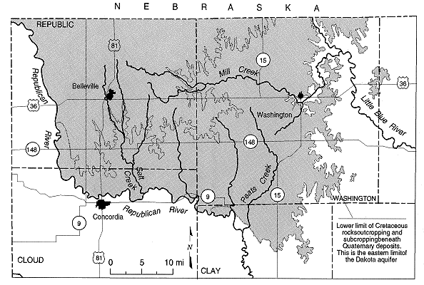
Figure 20. Location of the Cloud, Lincoln, Hodgeman, and Finney county monitoring sites in the Dakota aquifer of Kansas.
Cloud County Monitoring Site
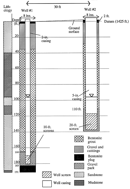
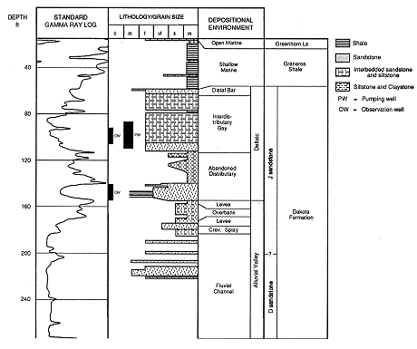
A monitoring site was established in NE NW NW sec. 7, T. 5 S., R. 1 W., Cloud County, to determine aquifer properties by means of pumping and slug tests. The site consists of two observation wells and a pumping well screened in the upper part of the Dakota aquifer. Initially, a 5-in. test hole was drilled using mud rotary to a depth of 293 ft. Gamma-ray and driller's logs of the deepest hole provide a detailed profile of the subsurface geology of the monitoring site (Figure 21). No significant sandstone was encountered below 190 ft. The test hole was backfilled with cuttings up to 191 ft and reamed to a diameter of 8 in. from land surface to 191 ft. It was then sealed with a bentonite plug up to 183 ft (Figure 22). A 2-in. PVC piezometer was constructed above this depth, with a 10-ft screen and 17-ft gravel-packed interval at the base of a thick sandstone (Figure 22, well 1). A second piezometer was screened in the mudstone between 76 and 86 ft, but the mudstone proved to be unsaturated at this depth and this piezometer was dry. An 8-in. hole was drilled to 139 ft for well 2 (Figure 22). This well was constructed with a 5-in. PVC casing so that it could be pumped using a submersible pump. It was screened over a 20-ft interval in the upper part of the same sandstone body at the same level in the aquifer as well 1.
Figure 21. Log of the test hole at the Cloud County monitoring site (NE NW NW sec. 7, T 5. S., R. 1 W.) showing lithologies and depositional environments. Lithologic types are from sample descriptions. The grain-size scale ranges from mud on the right to medium-grained sandstone on the left.
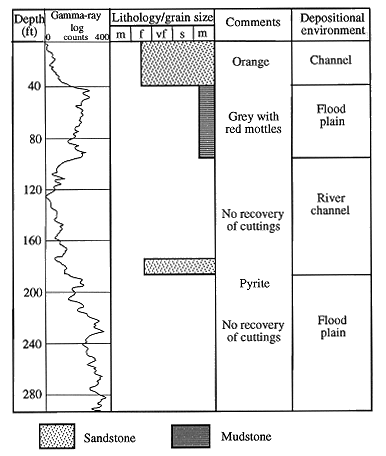
Figure 22. Monitoring and pumping well construction at the Cloud County monitoring site (NE NW NW sec. 7, T 5. S., R. 1 W.).
Lincoln County Site
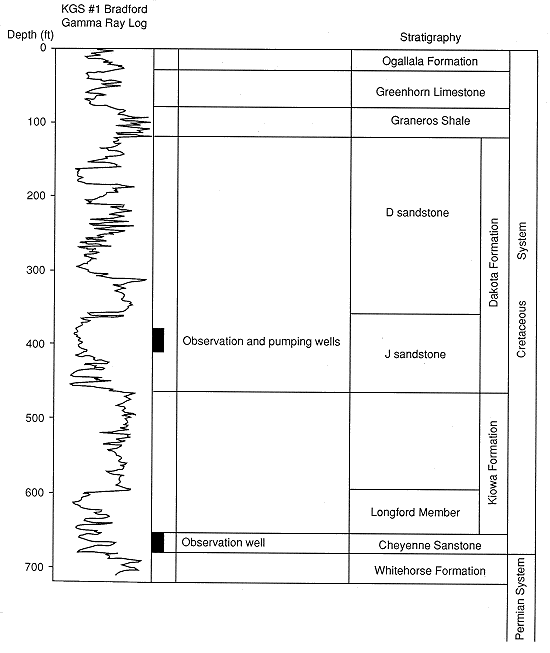
The Lincoln County monitoring site is located in NE NE NE sec. 2, T. 10 S., R. 8 W., approximately 300 ft west of the site of the KGS No. 1 Jones test hole. Construction took place in late October 1990. Figure 23 is a log of the upper part of this test hole in the upper Dakota Formation from core samples and the gamma-ray log from the No. 1 Jones. The monitoring and pumping wells were completed in the upper part of the Dakota Formation (upper Dakota aquifer). Two 2-in.-diameter PVC-cased monitoring wells and a 4-in.-diameter PVC-cased pumping well were installed at this site. The two observation wells were placed 20 ft away from and on opposite sides of the pumping well. The deep and shallow observation wells were screened between 135 ft and 145 ft and between 82 and 92 ft, respectively, below land surface. The pumping well was screened between 76 ft and 96 ft below land surface. Figure 24 shows the placement of the well screened intervals for the pumping and the observation wells. Each piezometer and the pumping well screen were gravel packed. The wells were developed by air to lift the drilling mud and water out of the well bore until the produced water from each of the piezometers and the pumping well was mud-free and the yield from the well was stable. Unfortunately, problems were encountered with the deep piezometer during development and repeated attempts to produce significant quantities of mud-free water met with failure.
Figure 23. Log of the test hole at the Lincoln County monitoring site (NE NE NE sec. 2, T 10. S., R. 8 W.) showing lithologies and depositional environments. Lithologic types are from sample descriptions. The grain-size scale ranges from mud on the right to medium-grained sandstone on the left.
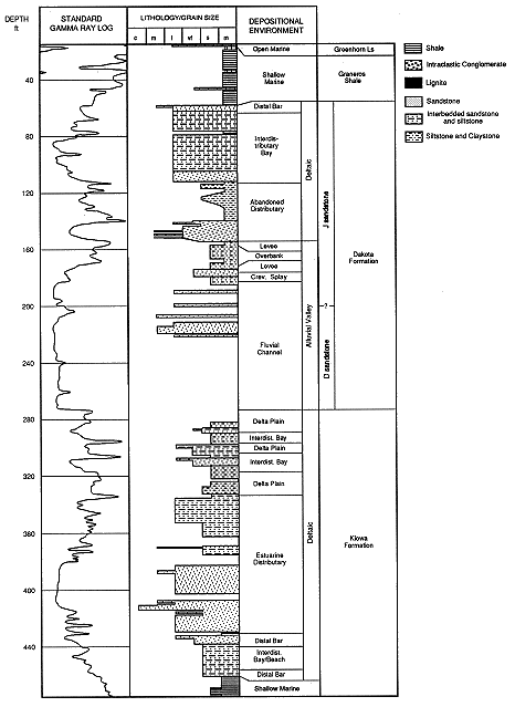
Figure 24.Placement of the monitoring (OW) and pumping well (PW) well screens at the Lincoln County monitoring site (NE NE NE sec. 2, T 10. S., R. 8 W.).
Hodgeman County Site
The monitoring site in Hodgeman County is located in NW NW SE sec. 29, T. 23 S., R. 23 W. Clarke Well and Equipment, Inc., of Great Bend, Kansas, constructed the monitoring wells between mid-April and mid-May 1991. A 2-in.-diameter and a 3-in.-diameter PVC-cased piezometer and one 5-in.-diameter PVC-cased pumping well were installed at the site. Figure 25 is a log of the piezometer borehole in the Cheyenne Sandstone (the deep piezometer) showing the location of the screened intervals at the monitoring site. The deep and shallow observation wells were screened between 653 ft and 683 ft and between 380 ft and 410 ft, respectively, below land surface. The pumping well was screened in the Dakota Formation between 380 ft and 410 ft.
Figure 25. Geophysical log of the deep (Cheyenne) piezometer borehole at the Hodgeman County monitoring site located in NW NW SE sec. 29, T. 23 S., R. 23 W., showing the placement of the screened intervals of the monitoring and pumping well.
As part of the study of the geology of the well site all electric well logs of the Dakota section within a nine (three by three) township area around the site were correlated in detail. Horizons correlated include the tops of the eroded Permian, the Cheyenne Sandstone, the Longford Member of the Kiowa Formation, the Kiowa Formation, the J sandstone interval (Dakota Formation), a lower D and an upper Dakota D sandstone interval (Dakota Formation), the Graneros Shale, and the Greenhorn Limestone. Structure and thickness maps of each interval were constructed based on the log picks. Computer-generated sand content values were read from the digitized logs, and sand percentages of the intervals were mapped. A set of cross sections using the digitized logs detail the stratigraphic variations of the Dakota aquifer around the well site.
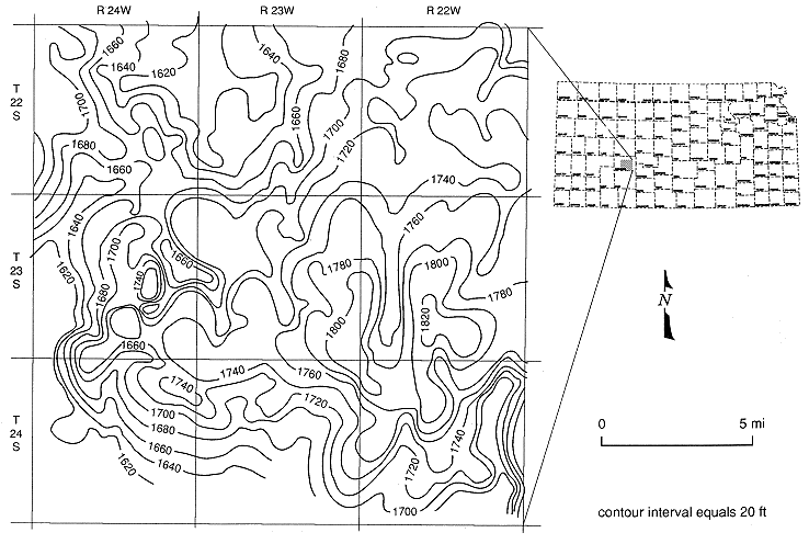
The series of structure maps show a paleoridge running east-west across southern Hodgeman County (Figure 26). This paleotopogaphic high was a drainage divide during Dakota deposition and influenced sandstone distribution patterns throughout Dakota sedimentation. The magnitude of the paleorelief of this area diminished from pre-Cheyenne time until the time ending Graneros deposition. The land surface at the initiation of Cheyenne deposition (Figure 26) reflected the topographic response to dissolution of buried Permian Flower-pot salt and the effects of erosion during the Jurassic and Lower Cretaceous. The Cheyenne Sandstone was deposited by rivers flowing generally from the east and around and off the drainage divide. The deposition occurred as a reaction to the slowly encroaching sea.
Figure 26. Elevation of the top of the eroded Permian surface around the Hodgeman County monitoring site located in NW NW SE sec. 29, T. 23 S., R. 23 W., from gamma-ray logs of boreholes drilled for petroleum exploration and development.
Further rise of sea level resulted in shoreline deposition along paleotopographic highs and marine shale deposition across the now submerged Cheyenne. Falling sea level caused fluvial incision at the base of the J sandstones. Subsurface deposits in extreme western Kansas preserve evidence of this transgression as the Huntsman Shale. Another cycle of sea-level fall and rise led to the unconformity at the base of the D sandstone and the deposition of fluvial sandstone above the unconformity. As the sea continued to transgress, the more deltaic upper portion of the D sandstone interval was deposited and full submergence is recorded by the Graneros Shale deposits. The trend of the river valleys can be traced in the thickest accumulations of deposits of the Cheyenne, J sandstone, and D sandstone sections. The marine infilling of lows and the overlapping paleotopographic highs is indicated in the isopachs of the Kiowa marine shale facies and Graneros Shale.
The sand percentage maps demonstrate the lateral variation and horizontal discontinuity of sand deposition across a fluvial valley. The vertical continuity of reservoirs is assured only in areas of stacked 100% sandstone intervals, which are rare; chances of interconnections of superimposed channel-fill deposits increase with increasing sandstone percentage.
The Hodgeman County monitoring site is located along a long-lived drainage system that flowed to the north and west off the Hodgeman County paleotopographic high. Several stacked Cheyenne channel sandstone deposits occur in the 655-682-ft interval of the deep monitoring well (Figure 25). The transgressive, deltaic, and shoreline deposits of the Longford Member of the Kiowa Formation are the sandstones between 598 ft and 652 ft in the log of the deep borehole. The deep marine Kiowa marine shale facies occurs between 466 ft and 598 ft; it is an effective aquitard when present. The fluvial-valley-fill deposits of the J sandstone are between 362 ft and 466 ft in the deep borehole electric log. The lower D sandstone fluvial deposits contain mostly overbank clays (310-362 ft. in the deep borehole well log). The marine-influenced transitional and deltaic sandstones of the upper D sandstone are at 188-310 ft on the well log, and the blanketing Graneros Shale lies between 76 ft and 118 ft (Figure 25).
Before drilling, preliminary depth, thickness, and sand content maps were constructed to test predictive capabilities of the mapping process. The actual depth, thickness, and sand content of the three aquifer units (Cheyenne, J sandstone, and D sandstone) were within 5% of the predicted values. Detailed mapping and interpretation of depositional systems allows this type of accuracy. A more regional interpretation pinpoints trends and probable aquifer presence.
Finney County Site
The U.S. Geological Survey (USGS) contracted for the drilling and development of pumping and monitoring wells in the lower part of the Dakota aquifer by Clarke Well and Equipment, Inc., of Great Bend, Kansas. The well was completed in SE SW SW sec. 9, T. 24 S., R. 33 W., Finney County, and has been assigned a well identification number, 24S-33W-09CCD4 by the USGS. This new well is located 30-40 ft from long-term observation wells installed by the KGS and USGS in 1977 and 1980 in the Dakota, Ogallala, and Arkansas River alluvial aquifers. The contractor installed a screened well at a finished depth of 494 ft after backfilling the hole from the drilled depth of 521 ft. The pumping well is a 5-in.-diameter PVC-cased well, 494 ft deep, screened with 40 ft of 0.030-in. mill-cut slotted PVC screen, and filter packed with coarse sand from 449 ft to 494 ft. The annular space above the filter pack is sealed with polymer gel and neat cement up to 360 ft, backfilled with sand from 360 ft to 368 ft, and sealed with bentonite, neat cement, and cement grout to the surface. Two feet of 5-in. PVC casing, plus cap, were left standing above land surface.
The field testing program at each site lasted about one month. The general procedure was to begin monitoring at a site 10 days to 2 weeks before a planned pumping test. Ground-water levels were monitored with electronic pressure transducers, and atmospheric pressure was monitored with an electronic barometer. Both the transducers and the barometer were connected to a data logger so that data could be recorded without the need for human intervention. Before placement at the site, the transducers and barometer were calibrated at the Kansas Geological Survey.
This initial period of monitoring was designed to gather information about background water levels at the site and to help define the relationship between barometric pressure variations and water level fluctuations. An understanding of the relationship between barometric pressure and water levels is necessary to correct the drawdown data measured during the pumping test for any changes in atmospheric pressure that might occur during the test.
A series of slug tests is performed before the pumping test. These slug tests allow some preliminary estimates of the subsurface flow properties at the site to be determined. These preliminary estimates are then used to plan the mechanics of the pumping test. Without the information from the slug tests, it would be difficult to estimate a pumping rate that would produce measurable drawdown at the observation wells but a drawdown at the pumping well that would not allow the water level to be drawn down beneath the intake screen of the pump.
After a ten-day to two-week period of background monitoring, a pumping test lasting approximately 24 hours is performed at each site. The well is pumped at a constant rate and drawdown is measured in both the pumping and observation wells during this test. In addition to the transducers and barometer, an electronic flowmeter is employed in order to closely monitor the rate of pumping throughout the test.
A final 10-day to 2-week period of monitoring follows the pumping test. The purpose of the monitoring is to assess the recovery of water levels after the period of pumping and to gather further information about the relationship between water-level fluctuations and atmospheric pressure changes. At the end of the period a final series of slug tests is performed to assess how the pumping changed the estimates of flow properties obtained from the earlier slug tests.
The program of slug tests carried out at each site is based on methods recently developed at the KGS. The slug tests are performed using the KGS packer-based slug test system. In this system an inflatable rubber packer is lowered into the well on pump rods. The packer is placed below the static water level in the well but above the well screen. It is then inflated from the surface using nitrogen gas, closing off the annular space between the inner diameter of the well and the original outer diameter of the uninflated rubber packer. The central pipe on which the packer is mounted is the only connection between the screened and the cased portions of the well. This pipe can be opened and closed using a brass plug that is attached to the pump rods. A slug test is initiated by closing off the central pipe and introducing a slug into the region above the packer. That slug is then introduced into the well screen by opening the central pipe. The water-level response to the introduced slug is measured with a pressure transducer placed above the packer.
After the slug test, the data are analyzed with an automated well-test analysis package (SUPRPUMP), recently developed at the KGS, to obtain estimates of the transmissivity and storativity of the formation in the vicinity of the well. Figure 27 displays the results of such an analysis for a well at the Lincoln County test site.
Figure 27. Data and fitted model results for a slug test performed at Lincoln County site. Note the high correlation between the estimated transmissivity and storativity parameters.
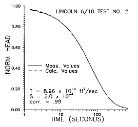
Research at the KGS has shown that conventional slug tests provide reasonable estimates of the formation transmissivity but poor estimates of the formation storativity. The reason for this is that there is relatively little information about the storativity in the recovery data measured at the slugged well. The little information that does exist is highly correlated with the information about the transmissivity of the formation. Thus it is difficult to estimate storativity independently from transmissivity. This condition produces the high parameter correlation shown in Figure 27, which will greatly influence the reliability of the estimated parameters. To improve the reliability of both the transmissivity and the storativity estimates obtained from a slug test, we introduced a new approach for the performance of slug tests as part of this project. In this approach data are collected not only from the slugged well but also from nearby observation wells. Figure 28 illustrates the results of such a test performed at the Lincoln County test site. An advantage of this approach is that there is considerably more information about formation storativity in the data measured at the observation well. In addition, this information is not highly correlated with information about the transmissivity of the formation. Thus the flow parameters can be estimated with much greater confidence than when only data from the slugged well are employed. A comparison of Figures 27 and 28 indicates how the parameter estimates will change with the addition of data from an observation well. Note that the observation well at the Lincoln County site was 21.17 ft from the slugged well. Theoretical modeling results indicate that an observation well more than 50 ft away from the slugged well could have been employed at this site. Clearly, slug tests in the Dakota aquifer are providing estimates of aquifer flow properties averaged over a much larger volume of the formation than is commonly recognized.
Figure 28. Data and fitted model results for the same slug test as in Figure 27. Observation well is 21.17 ft from slugged well. Note the significant decrease in parameter correlation that occurs when observation-well data are also included in the analysis.
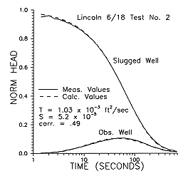
Figure 29. Geographic extent of the Republic, Cloud, Clay, and Washington county study area.
Geologic Framework
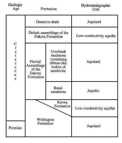
During FY89-90, eight test holes were drilled and logged in this area. The locations of these test holes are listed in the Dakota Aquifer Program: Annual Report, FY90. The test holes indicate that the aquifer consists of approximately 40% sandstone and 60% mudstone, mainly of the Dakota Formation. Interbedded sandstones and mudstones of the Kiowa Formation are also present in the subsurface in the western part of the study area but pinch out toward the east (Figure 30). Most of the sandstones were originally deposited in ancient river channels. They are generally continuous in a one-dimensional ribbon-like sense but not in a two-dimensional sheet like sense. However, there is a channel sandstone at the base of the Dakota Formation in all the test holes. Although this sandstone is unlikely to be present in an uninterrupted sheet throughout the study area, it is sufficiently continuous to be the most important conduit of lateral flow in the aquifer. The upper 25% of the Dakota Formation is composed of muddy sandstones and sandy mudstones deposited in a deltaic environment (Figure 30). Although this part of the formation is lithologically more homogeneous than the fluvial assemblage underlying it, the geohydrologic consequences of this greater continuity are offset because the deltaic sandstones are less permeable than the fluvial channel sandstones.
Figure 30. Stratigraphy and hydrostratigraphy of the bedrock in the Republic, Cloud, Clay, and Washington County study area.
Flow Systems
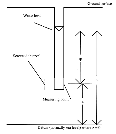
The hydraulic head h at a point in an aquifer is a measure of the potential energy per unit weight of the ground water at that point. It is easily measurable as the water-level above sea-level elevation in a well:
h = z + P, (1)
where z is the elevation of the measuring point and P is the pressure head (Figure 31). As the water moves through the aquifer, it flows from locations of high potential energy to locations of low potential energy. The direction of flow in a homogeneous aquifer is perpendicular to lines joining points of equal hydraulic head in the aquifer (equipotential lines). The water loses energy as it moves, and this is manifested as a drop in hydraulic head. The energy of the water is lost as frictional energy because of the resistance of the aquifer to flow.
Figure 31.Hydraulic head in a piezometer with its components of elevation head Z and pressure Y.
If the hydraulic heads in wells screened in a confined aquifer are plotted on a map and contoured with equipotential lines, the resulting map of the hydraulic head of the aquifer is termed the potentiometric surface of the aquifer. Because ground water in an aquifer flows from areas of high hydraulic head to areas of low hydraulic head, a map of the potentiometric surface can be a useful aid in understanding the directions of ground-water flow in different parts of the aquifer. It also helps to identify and illustrate zones of discharge and recharge and ground-water divides between flow systems.
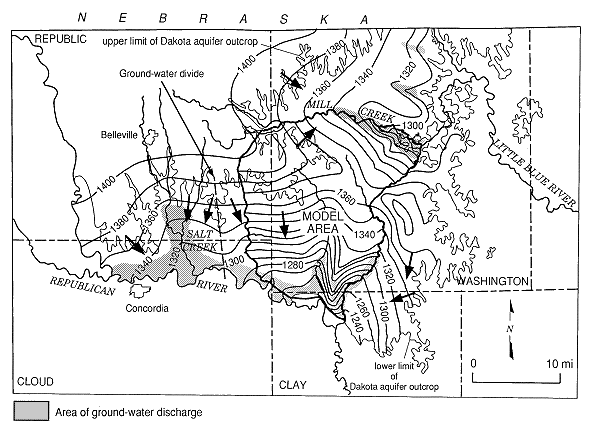
A potentiometric surface map of the basal sandstone in the study area was constructed in FY90. Figure 32 shows the directions of ground-water flow through this sandstone superimposed on the potentiometric surface. This information combined with hydrologic features of groundwater discharge, ground-water chemistry data, and topographic information was used to investigate the nature of the ground-water flow systems in the study area.
Figure 32. Potentiometric surface of the basal sandstone in the Dakota aquifer in the republic, Could, Clay, and Washington county study area with flow directions and ground-water discharge zones indicated. This figure also shows the location of the model area. Potentiometric contour interval is ten feet in the model area and 20 feet elsewhere.
There are three distinctive types of flow systems in hydrogeologic basins: regional, intermediate, and local (Figure 33). These flow systems are arranged hierarchically according to spatial and temporal scales in the ground-water basin. In local flow systems flow path length and ground-water residence time is small, whereas in regional systems these parameters tend to be large. Regional systems develop only where there is a general slope and local relief is negligible, and local systems develop only where there is pronounced local relief along the flow path. In most ground-water basins the flow system is gravity driven and the water table is a subdued replica of the land surface topography. Consequently, topographically elevated regions are zones of recharge, whereas topographically lower regions are zones of discharge in all three flow systems. In areas of ground-water discharge the hydraulic head is generally close to the land surface and there is an upward component to the flow direction. In discharge areas depth to water in wells decreases with increased well depth because of the upward vertical component of the hydraulic gradient. Common manifestations of ground-water discharge to the surface are seepage areas, springs, salt precipitates, relatively high mineralization of water, waterlogging and the presence of phreatophytes. Ground-water discharge zones generally occupy between 5% and 30% of the surface area of a watershed. In areas of ground-water recharge depth to water is large and there is a downward component to the flow direction. Depth to water in wells decreases with increased depth of the wells because of the downward vertical component of the hydraulic gradient.
Figure 33. Components of a hypothetical regional ground-water flow system in a homogeneous ground-water basin.
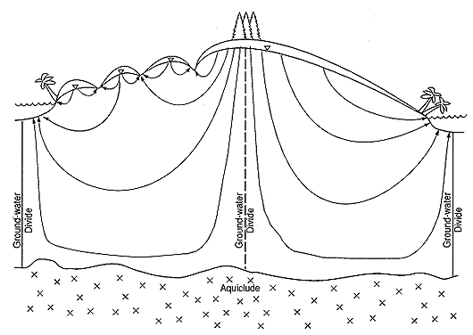
Mineralization of the water in recharge zones is relatively low. In general, the dissolved mineral content of ground water increases with residence time because of the longer contact time with the aquifer framework.
Application to the Dakota aquifer. The potentiometric surface for the basal sandstone of the Dakota aquifer was constructed using water levels from wells, topographic information and hydrologic features. Ground water flows through a combination of intermediate and local systems in the aquifer. Both types of system are ultimately driven by topography, although on different scales. The local flow systems are fueled directly by recharge from rainfall in upland areas within the study area. The intermediate flow system, which brings halite-solution brine into the study area from the west, is driven by the regional slope of the Great Plains toward the east.
Major zones of discharge from both types of system are in valleys that cut down to below the level of the hydraulic heads in the aquifer. Most of the discharge occurs along the contact with the alluvial aquifer in the Republican River valley and along the lower reaches of the south-flowing tributaries (Figure 32). Much of the flow in the regional flow system discharges in the watershed of one of these tributaries, named Salt Creek, in southern Republic and northern Cloud counties. East of this watershed, in southern Washington County, local flow systems predominate in the aquifer beneath south-flowing tributaries of the Republican River. Water in the local flow systems is pumped from the aquifer for domestic, irrigation, stock, and municipal use. In northern Washington County, in the Mill Creek watershed, most of the discharge from the aquifer is along Mill Creek and the lower reaches of its tributaries. Some saline water of the regional flow system discharges here also, although it is diluted by local recharge from above.
Modeling Efforts and Results
Determination of Recharge Rate. The recharge rate to a local flow system and the effects of pumping were investigated by simulating ground-water flow using MODFLOW. Flow was simulated in the sandstone at the base of the aquifer over a 300 mi2 area (Figure 34), which included the site of a pumping test performed in FY90. The basal sandstone is confined by mudstone throughout this area. The quality of the water is good; salinity is not a problem except in the northwestern comer of the model area, where brackish water has been reported in the basal sandstone. It was therefore hypothesized that within this area recharge from rainfall penetrates through leaky confining layers all the way down to the basal sandstone, and that this is the source of nearly all the water flowing horizontally through this sandstone. Although the hydraulic conductivity of mudstones is normally low, Darcian intergranular flow rather than flow through fractures is thought to be the way in which recharge makes its way down to the basal sandstone. Over a large area appreciable quantities of water can be transmitted in this way, despite a very low vertical hydraulic conductivity. To determine the recharge rate using a computer model, we assumed that the flow system was in a steady state. Although the aquifer is pumped at approximately 900 acre-ft/yr in the area of model A, there are no reports of significant declines of water levels and so the steady-state assumption is believed to be valid.
Figure 34. Model grid in the 300 mi2 area within the larger study area. The traces of the cross sectional models A and B are shown within the model area.
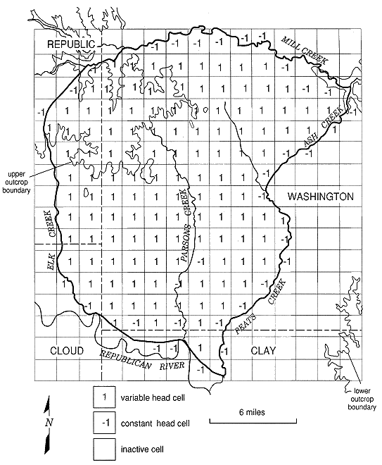
The model grid consisting of 240 cells (119 active, 88 inactive, and 33 constant-head cells) was constructed over the model area with square grid-cell dimension of 1.5 mi on a side (Figure 34). The head at the center of each cell was interpolated from the potentiometric surface map. The constant-head cells along stream boundaries were used to simulate ground-water discharge into streams and alluvial aquifers; some constant-head cells in the northwest corner and along the eastern edge of the model area simulated horizontal inflow at these boundaries. The grid-cell size was small enough to represent the locations of boundaries with reasonable accuracy but not too small for the density of field water-level data used to construct the potentiometric surface.
The head distribution in an aquifer in a steady state is dependent on the recharge rate and the transmissivity of the aquifer (transmissivity is the product of hydraulic conductivity and thickness). The hydraulic conductivity used in the simulation was estimated from a pumping test conducted in FY90. Thickness of the basal sandstone in this area was estimated from well-drillers' logs and KGS test holes.
The recharge rate in the simulation was varied until the minimum difference was found between simulated heads generated by the model and heads interpolated from the potentiometric surface. The simulated heads most closely matched the interpolated heads with a recharge rate to the basal sandstone in this area of approximately 0.26 in./yr. This recharge rate is reasonable, considering the precipitation, potential evapotranspiration, and vertical hydraulic conductivity of confining layers in the area. Recharge from above accounted for 83% of the total inflow into the system, lateral inflow from the east accounted for 12%, and lateral inflow from the west accounted for just 5%. A few miles to the west of the model area the aquifer is occupied by halite-solution brine of the intermediate flow system. Therefore the low proportion of inflow from the west in relation to the proportion of local recharge is the reason why water quality in the model area is good.
Cross-sectional simulations of flow in the aquifer along sections B and C (Figure 34) were also run within the area of model A. These simulations showed that consideration of an upper sandstone aquifer layer and intervening mudstone aquitard did not significantly affect the model A estimate of recharge rate to the basal sandstone.
Determination of the Effects of Pumping. The areal model was used to investigate the effects of pumping water from the aquifer on ground-water quality and availability, assuming a uniform recharge rate of 0.26 in./yr. To run this transient simulation, we needed an estimate of the storativity of the aquifer for each grid cell in addition to the model inputs. The storativity of a confined aquifer is the product of its specific storage and thickness. Specific storage throughout the model area was estimated from the pumping test conducted in FY90. The thickness of sandstone contributing water to the wells was estimated for each cell from well-drillers' logs and KGS test holes.
The current rate of ground-water withdrawal from the aquifer in the model area was estimated from individual irrigation-well appropriations from the Division of Water Resources (DWR). Irrigation wells account for over 90% of the water pumped from the Dakota aquifer in the model area; the remainder are domestic and stock wells. The mean annual DWR estimate of water use was found for each well for which there are existing records. Total water use from a group of irrigation wells in Washington County, including those in secs. 16-17, T. 5 S., R. 1 E. (Table 1), is substantially less than the total estimated by the DWR. Actual pumpage was 78% of the DWR estimate of pumpage. Therefore the water-use estimates for unmetered wells listed in Table 1 are 78% of the values determined directly from DWR water-use data. For irrigation wells with no known record, a pumping rate of 47 acre-ft/yr was estimated. This is the mean rate of water withdrawal from the wells that do have records.
In addition to the high-capacity wells listed in Table 1, there are records of 70 domestic and stock wells screened in the basal sandstone in the model area. If these were all pumped at 300 gallons per day, the total annual pumpage from domestic wells would be no greater than 25 acre-ft. In addition there is probably a similar number of low-capacity wells, such as old windmill wells, that are in use but that have no official records. The total annual pumpage from these wells is also likely to be no greater than 25 acre-ft. The total annual pumpage from all low-capacity wells in the basal sandstone was therefore estimated to be 50 acre-ft, which is approximately equivalent to the annual pumpage of one typical irrigation well.
Current rates of ground-water withdrawal were simulated using the well package of MODFLOW. The estimated ground-water withdrawal of 754 acre-ft from high-capacity wells was applied to the relevant grid cells (Table 1). Withdrawals attributed to low-capacity wells were evenly distributed throughout the active nodes of the model.
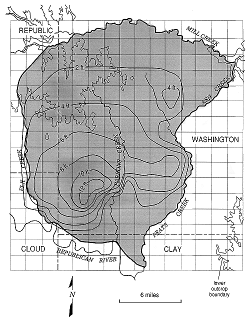
Simulated pumping of the aquifer at this annual rate resulted in a mean drawdown of 2.1 ft in the area of the simulation after the system reached equilibrium (Figure 35). Pumping was assumed to be uniform throughout the year. In reality, pumping of high-capacity irrigation wells is seasonal and therefore the drawdown would vary from season to season. Lateral inflow from the west amounted to 6% of the total inflow into the system in the simulation. These results are compatible with the fact that no significant drops in water levels and no significant changes in water quality have been reported in this area.
Figure 35. Drawdown induced by pumpage at present rates in the basal sandstone of the Dakota aquifer in the model area in Republic, Cloud, Clay, and Washington counties. Drawdown contours have a two-feet contour interval.

Table 1. Current Ground-Water Use from the Dakota Aquifer in the Model Area of Washington, Cloud, Clay, and Republic Counties.
| Location | Grid cell (row, column) |
Number of wells |
Mean annual water-use estimate (acre-ft/yr) |
Source of estimate |
|---|---|---|---|---|
| sec. 26, T. 3 S. , R. 2 E. | 5,11 | 1 | 47 | estimated |
| sec. 36, T. 3 S., R 2 E. | 6,11 | 1 | 47 | estimated |
| sec. 24, T.4.S., R..2.E. | 9,11 | 2 | 81 | DWR, App. 1 |
| sec. 1, T. 5 S., R. 1 E. | 11,7 | 1 | 53 | DWR, App. 1 |
| sec. 10, T. 5 S., R. 1 E. | 11,6 | 2 | 136 | DWR, App. 1 |
| sec. 16, T. 5 S., R. 1 E. | 12,5 | 1 | 56 | DWR, App. 1 |
| sec. 17, T. 5 S., R. 1 E. | 12,5 | 3 | 124 | DWR, App. 1 |
| sec. 20, T. 5 S., R. 1 E. | 13,5 | 1 | 22 | DWR, App. 1 |
| sec. 30, T. 5 S., R. 1 E. | 13,4 | 1 | 47 | estimated |
| sec. 1, T. 5 S., R. 2 E. | 10,11 | 2 | 94 | DWR, App. 1 |
| sec. 12, T 5 S, R 1 W | 11,3 | 1 | 47 | estimated |
| Total | 16 | 754 |
Doubling the pumping rate had the effect of doubling the mean drawdown in the model area to 4.3 ft and of inducing mean drawdowns of over 13 ft in the areas of highest use (Figure 36). Drawdowns of this magnitude would reduce the yields of wells because of the greater vertical distance through which pumps would need to lift the water. Lateral inflow from the west was not appreciably increased by doubling the pumping rate.
Figure 36. Drawdown induced by pumpage at double the present rate in the basal sandstone of the Dakota aquifer in the model area in Republic, Cloud, Clay, and Washington counties. Drawdown contours have a two-feet contour interval.
In summary, the Dakota aquifer can sustain the current level of pumping in the 300 mi2 area of the model without adversely affecting water quality or availability. Doubling the pumping rate in this area would likely substantially lower the water level in the aquifer in the areas of highest use but would not produce severe water-level declines in the aquifer in general or adversely affect water quality. The prediction of the effects of increased use is not applicable in other parts of the study area, particularly west and north of the model area, where salinity of the ground water is already a problem.