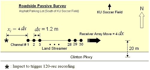
Passive Roadside MASW
This is a passive mode of survey that can be implemented with a conventional linear receiver array (Figure 1). Although it can result in a certain degree (usually less than 10%) of overestimated Vs values in comparison to the 2-D receiver array (Park and Miller, 2006), this survey mode can be useful and convenient because in field operations it does not require a large open area for receiver deployment. In fact, the survey can be repeated by progressively moving the receiver array by a certain distance along the road (the roll-along survey mode) so that a 2-D Vs profile can be obtained. Procedures of data acquisition and processing are explained.
Figure 1--Passive Roadside MASW method.
Receiver Array
A linear array deployed along a roadside is used. Although it does not have to be close to the road, it is recommended to maintain the offline distance (between the array and the road center) fairly constant (for example, within ±30%) throughout the entire survey.
Array Dimension (D) and Receiver Spacing (dx)
Array dimension (D) is directly related to the longest wavelength (![]() ) that can be analyzed, which in turn determines the maximum depth of investigation (zmax):
) that can be analyzed, which in turn determines the maximum depth of investigation (zmax):
![]()
On the other hand, (minimum if uneven) receiver spacing (dx) is related to the shortest wavelength (![]() ) and therefore the shallowest resolvable depth of investigation (zmin).
) and therefore the shallowest resolvable depth of investigation (zmin).
![]()
Data Acquisition
The following describes most of parameters related to data acquisition. These are the parameters most commonly used at KGS and by no means represent a required set of values. A slight variation in any parameter can always be expected.
Recording Parameters
Sampling interval of 4 ms (dt = 4 ms) and total recording time of 30 sec (T = 30 sec) are most commonly used at KGS when surveys are performed inside the city of Lawrence. Total recording time (T) is determined in such as way that there is at least one occurrence of passive surface wave generation during recording. Therefore, it can be reduced or increased depending on local situations related to the surface wave generation. In case of surveys near roads, for example, there should be a vehicle passing near the survey area at least once during recording.
The longer T is not always better. This is because the chance of recording surface waves generated at different locations on the road increases as well and it will in general degrade the data processing resolution unless those locations are well apart in azimuth (for example, 90° or more). If the main source point is fixed in location, however, the longer T will be the better. A fixed source point of major surface waves is observed when you hear a loud jolting sound coming from nearly the same spot on the road as vehicles pass over.
Vertical stacking during recording is strongly discouraged (unless T is significantly limited) because it will increase the change of recording multi-azimuth surface waves explained previously. Instead, we recommended saving individual records separately. Then, the dispersion imaging process can be applied to individual records and then these image records can be vertically stacked together to enhance the definition of the image. However, if T is limited to a shorter time (e.g., < 30 sec) by the recording device, then a few times of vertical stacking (e.g., stacking 10-sec recording three times) may be necessary either during recording or post-acquisition stage
D and dx will approximately determine the minimum number of channels needed. In any case, however, more channels will be an advantage that can increase the resolution of dispersion processing to a certain degree. 48 channels are most desirable for a survey aiming at zmax ≈ 100 m. When fewer than 48 channels are available (e.g., 24), data acquisition can proceed with an array of smaller dimension (e.g., D = 25 m) and then with progressively larger dimensions (e.g., D = 50 m, 75 m, 100 m, etc.) to cover a broader range of wavelengths (![]() ). In this case, dispersion image data sets processed separately can be combined together to construct a broader-band dispersion image. Because of the 1-D nature of the array, usually 24-channel acquisition may be used to aim at zmax=100 m with dx=5 m. A 48-channel acquisition, however, will be advantageous with an increased resolution in data processing especially at higher (shallower) frequencies (depths).
). In this case, dispersion image data sets processed separately can be combined together to construct a broader-band dispersion image. Because of the 1-D nature of the array, usually 24-channel acquisition may be used to aim at zmax=100 m with dx=5 m. A 48-channel acquisition, however, will be advantageous with an increased resolution in data processing especially at higher (shallower) frequencies (depths).
If dynamic range is a controllable option with a recording device, choosing the highest value, along with the highest gain if available also, will always be a benefit.
Necessity of Separate Active Survey
Instead of a separate active survey, use a sledge hammer to apply an impact at one specific (inline) distance away from one end of the array to trigger recording of, for example, a 30-sec long record (Figure 1). Then, take the earliest a few seconds (for example, 0-2 seconds) of record at the beginning of data processing to make a separate active data set, and use the rest of the record (for example, 2-30 seconds) for the passive data set as explained in the Data Processing section following. In this case, analyzed Vs information at shallow depth will be biased towards the impact location.
Data Processing
Step 1: Format (conversion from SEG-2 to KGS format)
Step 2: Splitting Data into Active and Passive Sets
Because an active impact is applied at the beginning of long (for example, 30-sec) recording, the early portion of data contains active surface waves that can be processed by the normal active processing procedure, whereas the later portion contains passive surface waves. As processing schemes are different for active and passive cases, they have to be separated to avoid adverse influence on each other. Usually the first 2-sec portion is enough to take most of the active surface waves.
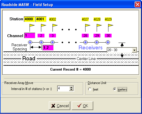
Step 3: Field Setup
Active (Figure 2) and passive (Figure 3) portions of data set are encoded through separate procedures. Station numbers are arbitrary fictitious numbers used as reference surface coordinates. However, station numbers should match between active and passive portions of data so that their dispersion images can be combined appropriately.
Figure 2--Setting up active portion of the acquisition.
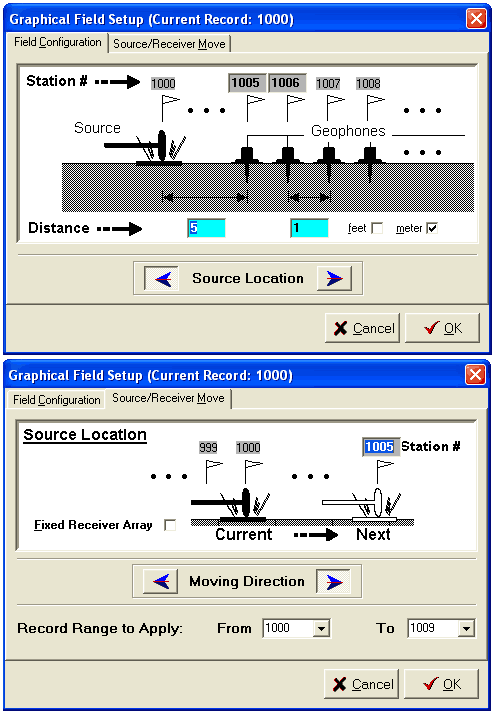
Figure 3--Setting up passive roadside portion of the acquisition.
Step 4: Generation of Dispersion Image (called overtone) Data
Process active and passive data sets separately.
Step 5: Combining Active and Passive Overtone Data Sets
Step 6: Extraction of Dispersion Curve(s)
Step 7: Inversion of Curves for 2-D Vs Profile
References
Park, C.B., and Miller, R.D., 2006, Roadside passive MASW: Proceedings of SAGEEP, April 2-6, 2006, Seattle, Washington. [PDF available online, 1.3 MB]