![]()
Prev Page--Unconsolidated Aquifers || Next Page--References
Ground-water Development
Irrigation has been practiced in Scott County on a small scale since about 1650 when the Taos Indians diverted water from Ladder Creek to irrigate crops in an area near the present Lake Scott. Pumping ground water for crops was practiced as early as 1888. By 1895, 24 individuals were reported to be irrigating a total of 40 acres (16 hm2) (McCall, 1944). All the power was supplied by windmills and each well probably irrigated little more than a garden plot. According to McCall (1944), the next phase of irrigation development began in 1908 when E. E. Coffin operated an irrigation plant that pumped about 120 gpm (7.6 L/s) using a centrifugal pump driven by a gasoline engine. Two new windmill plants were constructed in 1911 and 1912. Each windmill plant had several wells and a reservoir for storing water. In 1917, J. W. Lough, who was called the "father of pump irrigation in Scott County," completed a $75,000 plant for generating electricity to power his wells. This local electric plant used fuel oil for energy. Although definite information is not available, irrigated acreage in Scott County apparently reached a peak of about 5,000 acres (2,020 hm2) in 1922 and then declined steadily to a low of 1,020 acres (410 hm2) in 1932 (McCall, 1944). According to Pfister (1955), the extension of electric lines into the Shallow Water area in 1932 helped increase irrigated acreage to 4,000 acres (1,620 hm2) in 1934. Acreage remained nearly constant until 1937, when it increased during 1937-38 to 10,355 acres (4,190 hm2). The increase that started in 1937 was partly due to the extension of natural gas lines into the pumping district. The irrigated acreage for Scott County continued to grow, reaching 12,389 acres (5,010 hm2) in 1939. In 1945 a total of 129 wells supplied 18,400 acre-feet (23 hm3) of water to irrigate 21,000 acres (8,500 hm2) (Waite, 1947).
Irrigation development in Lane County was slower than in Scott County, as there were less than 500 acres (200 hm2) irrigated from three wells in 1949 (Prescott, 1951). From these meager beginnings, irrigation increased until 1972 when about 100,000 acres (40,470 hm2) were irrigated in Scott County and about 20,000 acres (8,090 hm2) were irrigated in Lane County. An average of 136 acres (55 hm2) per well are being irrigated in the two counties.
Location of Wells
As of January 1973, there were 164 large-capacity wells in Lane County and 717 large-capacity wells in Scott County. This total includes all irrigation, industrial, and municipal wells that yield 100 gpm (6.3 L/s) or more. Most of the wells have been drilled within the main body of the unconsolidated aquifer shown on plate 2. Wells in T. 18 S., R. 31 W. are in the chalk aquifer and wells in T. 20 S., R. 31 W. are in an isolated alluvial channel separated from the main body of the unconsolidated aquifer.
Irrigated Acreage
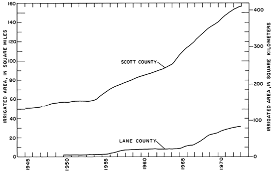
In 1972 about 20,000 acres or 31.2 square miles (80.9 km2) were irrigated in Lane County and about 100,000 acres or 156.2 square miles (404.6 km2) in Scott County (fig. 11). These data are from records of the Division of Water Resources, Kansas State Board of Agriculture. The data have been adjusted to account for duplication of the same acreage under more than one application. The graph shows that the amount of land under application to appropriate ground water has continued to increase rapidly since the middle 1960's.
Figure 11--Irrigated area according to Kansas State Board of Agriculture records, adjusted for duplication of areas under application.
As part of a study to improve accuracy and timeliness of information on land use, such as irrigated acreage, the Kansas Geological Survey is utilizing imagery acquired from the Earth Resources Technology Satellite (ERTS) [now referred to as LANDSAT]. Figure 12 is a portrayal of Lane and Scott Counties produced from imagery at an altitude of 570 nautical miles (1,054 km).
Figure 12--MSS Band 5 (red band) imagery of Lane and Scott counties from altitude of 570 nautical miles (1,054 kilometers). Imagery by NASA, Earth Resources Technology Satellite, Sept. 22, 1972.
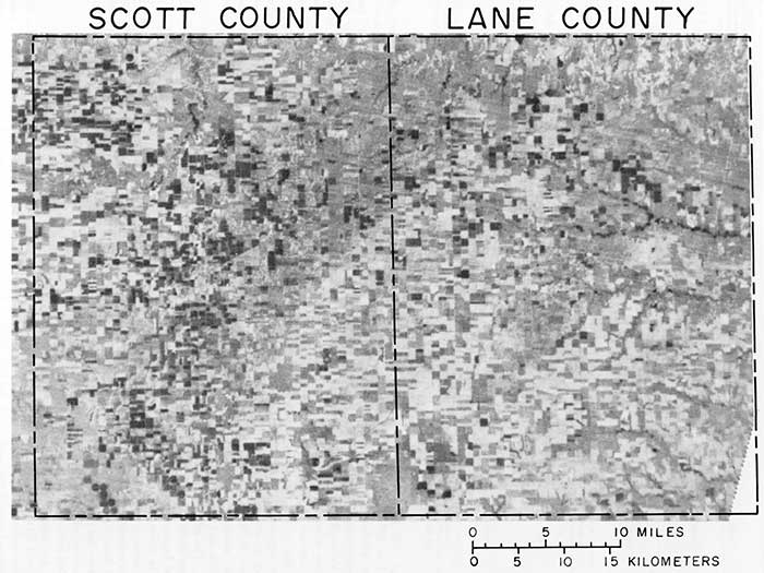
The drainage pattern of Ladder Creek in northwestern Scott County and the major forks of Walnut Creek and Hackberry Creek in eastern Lane County are seen as a sinuous pattern of dark gray-black tone where springs and seeps provide adequate moisture for phreatophyte growth. Outcrop areas of the Niobrara Chalk along the northern and eastern borders exhibit irregular patterns of light-gray tone.
The east-west orientation of fields is a means of reducing erosion by the predominant southerly and northerly winds. In general, medium- to light-gray tones are pasture land and fallow or stubble fields. Dark-gray tones represent untilled grass land illustrated by the sandhills in southwest Lane County and southeast Scott County. Dark gray-black tones are indicative of irrigated fields; the circular patterns of about 140 acres (57 hm2) are irrigated by center-pivot sprinklers. Two distinctive northeast trending dark-gray bands on the figure represent areas wetted by heavy thunder showers that occurred one week before the imagery was taken.
Annual Withdrawals
The quantity of water pumped can be estimated for those large-capacity wells for which power-consumption and pump-discharge data are available. Water pumped from the gas-powered wells can be estimated by dividing the total cubic feet of gas used by an appropriate power factor. Water pumped from the electric-powered wells can be estimated by dividing the total kilowatt-hours used by an electric-power factor.
The power factor (Kg) for natural gas was determined by measuring the discharge of the well, the rate of natural-gas consumption at that discharge, the line pressure at the meter, and applying the equation:
Kg = (1.955 × 10⁷ V Pg) / Q tg
where:
Kg = power factor measured in cubic feet of natural gas to pump 1 acre-foot of water (ft3 / acre-ft). Converting to metric units: Cubic meters of gas to pump 1 cubic hectometer of water (m3/hm3) = 23 Kg,
V = cubic feet of natural gas consumed in tg seconds,
Pg = pressure factor,
Q = pump discharge, in gallons per minute,
tg = time, in seconds, to consume V cubic feet of natural gas.
The pressure factor (Pg), furnished by the gas company, is a function of atmospheric pressure, altitude above sea level, and gas-line pressure. It is used to standardize the amount of gas consumed.
The electrical power factor (Ke), representing the amount of electricity required to pump an acre-foot of water in the study area, was determined by applying the equation:
Ke = (1.955 × 10⁴ R Kh) / Q te
where:
Ke = power factor measured in kilowatt-hours to pump 1 acre-foot of water (Kwh/ acre-ft) Converting to metric units: Kilowatt-hours of electricity to pump 1 cubic hectometer of water (Kwh/hm3) = 810 Ke;
R = revolutions of meter disc in t, seconds,
Kh = constant for each meter (generally stamped on the nameplate of the instrument) giving the number of watt-hours represented by one revolution of the meter disc,
Q = pump discharge, in gallons per minute,
te = time, in seconds, for meter disc to make R revolutions.
To estimate the annual withdrawals from the area, fuel and power records were obtained from KansasNebraska Natural Gas Company, Inc., Lane-Scott Electric Cooperative, and Wheatland Electric Co-op, Inc. Power consumption mainly varies with differences in pump efficiency, pump discharge, discharge pressure, and depth to water. Values of Kg for 22 wells ranged from 3,800 to 13,000 ft3/acre-ft (87,000 to 299,000 m3/hm3) with a median value of 5,600 ft3/acre-ft (129,000 m3/hm3). The median K, value for 8 wells is 417 Kwh/acre-ft (338,000 Kwh/hm3) with a range of 219 to 555 Kwh/acre-ft (177,000 to 450,000 Kwh/hm3).
Approximations of ground water pumped by natural gas and electricity were computed by applying the median values of Kg and Ke to the total power consumed in the counties for the years 1971 and 1972 as tabulated in table 5. The total annual pumpage of all wells in the two-county area may be extrapolated by assuming that the average amount of water pumped per well by natural gas or electricity equals the average amount of water pumped per well by all fuels. Data in table 5 show a total pumpage of about 180,000 acre-feet (220 hm3) in 1971 and 120,000 acre-feet (150 hm3) in 1972. The greater amount pumped in 1971 and the lesser amount pumped in 1972 are attributed to below-normal and above-normal precipitation during the growing season respectively, although annual precipitation for both years was above normal (See table 6).
Table 5--Power consumption and calculated pumpage for Lane and Scott Counties for 1971 and 1972. (e) denotes extrapolated elata.
| Year | County | Type of power |
Percent of wells |
Power consumption |
Calculated water pumped (acre-ft) |
Estimated irrigated acres |
Water applied annually (ft/acre) |
|---|---|---|---|---|---|---|---|
| 1971 | Lane | Natural Gas | Assumed same as 1972 |
143,208,300 Ft3 | 25,600 | 19,000 | 1.6 |
| Electricity | 1,115,866 Kwh | 2,700 | |||||
| Other (e) | 2,100 | ||||||
| Total | 30,400 | ||||||
| Scott | Natural Gas | Assumed same as 1972 |
740,473,000 ft3 | 132,000 | 98,000 | 1.5 | |
| Electricity | 3,652,304 Kwh | 8,800 | |||||
| Other | 9,000 | ||||||
| Total | 149,800 | ||||||
| Summary for Lane and Scott Counties | 180,200 | 117,000 | 1.5 | ||||
| 1972 | Lane | Natural Gas | 61 | 117,387,000 ft3 | 21,000 | 20,000 | 1.2 |
| Electricity | 32 | 923,349 Kwh | 2,200 | ||||
| Other (e) | 7 | 1,700 | |||||
| Total | 24,900 | ||||||
| Scott | Natural Gas | 90 | 457,036,800 ft3 | 81,600 | 100,000 | 0.9 | |
| Electricity | 4 | 3,047,060 Kwh | 7,300 | ||||
| Other (e) | 6 | 5,700 | |||||
| Total | 94,600 | ||||||
| Summary for Lane and Scott Counties | 119,500 | 120,000 | 1.0 | ||||
Table 6--Precipitation (in inches ). [From Climatological Data, U.S. Dept. of Comm., Environmental Data Service.]
| Year | Healy | Scott City | ||||||
|---|---|---|---|---|---|---|---|---|
| Annual | April-September | Annual | April-September | |||||
| Total | Departure from norm |
Total | Departure from norm |
Total | Departure from norm |
Total | Departure from norm |
|
| 1971 | 20.87 | +2.22 | 11.23 | -2.93 | 20.05 | +.88 | 13.49 | -1.00 |
| 1972 | 27.31 | +8.66 | 22.40 | +8.24 | 27.91 | +8.74 | 22.47 | +7.98 |
The amount of water pumped in Scott County by natural gas in 1972 was about 38 percent less than in 1971 as opposed to only 18 percent reduction in pumpage by other methods in the two counties. This difference in Scott County is attributed to the fact that the natural-gas-powered wells generally have high yields and are closely regulated to dry and wet periods. The effect of precipitation on total pumpage from low-yielding wells, however, is not as pronounced because of the longer pumping periods required to cover the acreage being irrigated.
The amount of natural gas used to generate electricity is currently about 17 cubic feet (0.48 m3) per kilowatt-hour. The amount of natural gas required to generate the power for electric motors, when added to the amount of natural gas used directly by natural-gas-fueled motors, gives an approximation of the total natural gas consumed for irrigation. In 1971 a reported total (State Corporation Commission, 1973) of 778 billion cubic feet (22.0 billion m3) of natural gas was produced from 5,396 wells in all fields in southwestern Kansas. Natural-gas production averages about 400,000 cubic feet (11,000 m3) per well per day.
During 1971, 960 million cubic feet (27 million m3) of gas was used-880 million cubic feet (25 million m3) directly and 80 million cubic feet (2.3 million m3) for generation of electric power-to provide power for irrigation wells in Lane and Scott Counties. Thus, the 1971 gas-energy input for irrigation pumpage was 0.12 percent of the total natural gas produced in southwestern Kansas, which is equivalent to the production of about 6 typical gas wells. In 1972, the gas-energy input for irrigation pumpage was 0.08 percent of the total natural gas production in southwestern Kansas, or the production of about 4.5 typical gas wells.
Effects of Ground-water Development
The development of large quantities of ground water for irrigation in Lane and Scott Counties has caused a decline in water levels, a reduction in base flow of Ladder Creek, and a decrease in the amount of ground water in storage.
Water-Level Changes
The amount of water-level change associated with the development of ground water for irrigation can be determined by comparing data collected by Waite (1947) and Prescott (1951) to similar data collected in 1973. Water-level (head) declines in the period from 1940-48 to 1973 ranged from less than 10 feet (3 m) to about 50 feet (15 m), as shown on plate 3. The greatest declines, located in T. 18 S., R. 33 W.; T. 20 S., R. 32 W.; and T. 20 S., R. 33 W. on the flanks of the south-trending trough, are interpreted to be in areas where the aquifer has a low specific yield under confined conditions. The drawdown and lateral extension of the cone of depression must be greater under confined than under unconfined conditions to yield equal amounts of water. If the storage coefficient is assumed to be 0.15 for unconfined conditions and .001 for confined conditions, the unconfined aquifer would yield 150 times more water than the confined aquifer for the same water-level decline.
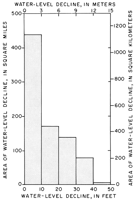
As pumping continues, water levels in the confined part of the aquifer may decline below the top of the principal water-yielding material. At that time water in the aquifer would become unconfined, and the rate of water-level decline decreases. As shown on figure 13, water levels declined less than 10 feet in about one-half of the area from 1940-48 to 1973. Declines greater than 30 feet occur in about 10 percent of the area underlain by the unconsolidated aquifer.
Figure 13--Areal extent of water-level declines from 1940-48 to 1973, in feet, in the unconsolidated aquifer.
Measurements in 46 wells in Scott County indicate that water-level declines averaged 1.15 feet per year (0.35 m/yr) during 1966-74 (Pabst and Jenkins, 1974). Water-level declines in wells throughout the two-county area underlain by the unconsolidated aquifer probably would average slightly less.
A long-term hydrograph (fig. 14) of water levels in observation well 18-33W-12add, located 1 mile (1.6 km) north of Scott City, is based on measurements provided by the Division of Water Resources, Kansas State Board of Agriculture. Because the observation well is in the vicinity of many irrigation wells, the hydro graph shows the response of water levels to seasonal pumping for irrigation. More importantly, however, the hydrograph shows long-term trends of water levels in the area. The period 1939-47 was one of slight decline, indicative of an area under early irrigation development. The period 1950 through the summer of 1952 was one of rising water levels culminating in the highest recorded water level on May 26, 1952. The rise is attributed to reduced pumping during a period of above-normal precipitation that recharged the aquifer and permitted artesian head to reach a high static level. Water levels declined as irrigation development accelerated during the drouth that lasted from mid-1952 to 1957. Recharge from precipitation caused a slight rise from 1957 to 1959, but declines in water levels during summer months show that pumping continued. The steadily declining water levels since 1960 are evidence of ground-water mining resulting from intensive irrigation development.
Figure 14--Hydrograph of observation well 18-33W-12add.
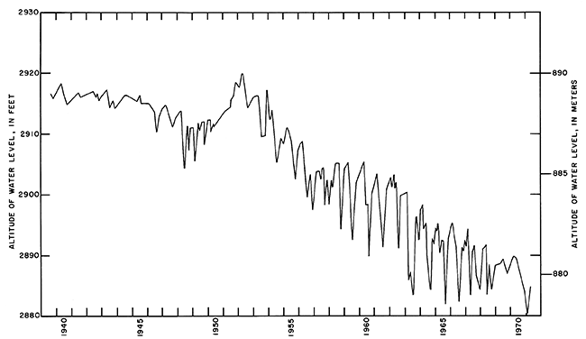
Observation well 18-33W-12add and the closest irrigation well are about 85 to 90 feet (26 to 27 m) deep. The seasonal fluctuations in the hydro graph may represent the effect of pumping from the closest irrigation well where water in the upper part of the aquifer is unconfined. The fluctuations may also represent, in part, pumping from other nearby irrigation wells that are about 180 to 220 feet (55 to 67 m) deep. It is possible, however, that the deep wells pump from the lower part of the aquifer where the water is semiconfined or confined beneath intercalated clay lenses. The net result of the ground-water mining has been the dewatering of the upper part of the aquifer as a direct response to withdrawals for irrigation.
Depletion of Ground Water in Storage
Depletion of ground water in storage is indicated by water-level declines resulting from irrigation development. To relate the long-term effects of irrigation withdrawals to changes in ground-water storage, the water-level declines during 1940-48 to 1973 are illustrated in plate 3 as a percent of change from the 1940-48 saturated thickness. The percent decline in saturated thickness with respect to area is graphically summarized in figure 15. Throughout most of the main body of the unconsolidated aquifer, the saturated thickness has been reduced by an amount ranging from 10 to 60 percent. Saturated thickness in two areas has been reduced 100 percent, and the aquifer is dewatered.
Figure 15--Areal extent of water-level declines from 1940-48 to 1973, in percent of saturated thickness of the unconsolidated aquifer.
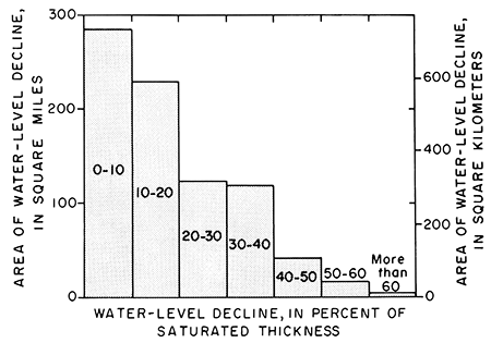
The significance of the water-level decline can be determined by comparison of the areal distribution of water-level changes and the percent change in saturated thickness. For example, the saturated thickness at Scott City was about 185 feet (56 m) during 1940-48. By 1973, a decline in water levels of 30 feet (9 m) reduced the saturated thickness to about 155 feet (47 m)--a reduction of about 16 percent. The saturated thickness in T. 18 S., R. 34 W. (an area of extensive development) was about 60 feet (18 m) during 1940-48. By 1973, a decline in water levels of 30 feet (9 m) reduced the saturated thickness to about 30 feet (9 m)--a reduction of about 50 percent. The effect of water-level declines has been a reduction in well yields and an increase in the cost of pumping.
Assuming that the specific yield is about 15 percent where the water is unconfined and about 1 percent where the water is semiconfined or confined, the annual reduction of ground-water storage in Scott County is estimated to be about 57,000 acre-feet (70 hm3) for the period 1966-74. This value for reduction in storage, based on water-level declines, is comparable to the 101,000 to 47,000 acre-feet (125-128 hm3) estimated from the ground-water inventory for 1971 and 1972, respectively.
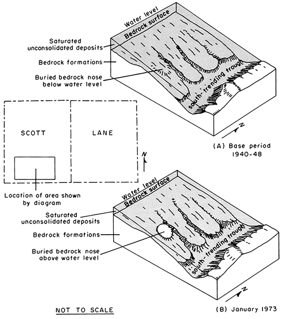
An extreme example of ground-water depletion is illustrated by the diagrammatic sketch (fig. 16) showing a generalized section across the southwestern part of Scott County, where a thin saturated area that overlies a bedrock nose on the west side of the deep south-trending trough and is adjacent to an area of intensive pumping has been completely dewatered. The exact amount of water-level decline and the time when the decline occurred are not known, but in at least part of the area the saturated thickness has decreased by 100 percent (pI. 3). There is no evidence that deposits overlying the bedrock high east of the deep south-trending trough ever were saturated.
Figure 16--Effects of water-level decline in the vicinity of a bedrock nose, southwestern Scott County.
Future Outlook for Irrigation
Potential Yields
Potential yield is defined as the yield that can be expected when the water-level drawdown in the pumped well is equivalent to 70 percent of the effective thickness of the aquifer. The effective thickness, which is comprised of those parts of the aquifer material yielding most of the water to wells, probably is the most important factor in estimating well yield. Effective-thickness computations for the sites where large-capacity wells were tested, amount to 80 percent or more of the total saturated thickness. Effective thicknesses at most irrigation wells are greater than 20 feet (6 m). Where the saturated thickness and effective thickness are known, an estimated potential-yield value can be based on the median specific-capacity value of 18 (derived from well-production tests shown on table 3) multiplied by the proposed drawdown. For example, a site that is underlain by 40 feet (12 m) of saturated thickness and contains 32 feet (10 m) of water-yielding material has 80 percent effective thickness, which is typical of irrigation wells in the area. The estimated potential yield at this site, computed by multiplying the drawdown of 22 feet (7 m) or 70 percent of the effective thickness by the median specific-capacity value of 18, would be about 400 gpm (25 L/s).
Potential yield to irrigation wells in the unconsolidated aquifer in Lane and Scott Counties ranges from less than 250 gpm to greater than 1,000 gpm (16 to 63 L/s). Plate 3 shows the potential well yields that can be expected in the unconsolidated aquifer in the two-county area. Data from existing wells, well-production tests summarized in table 3, saturated thickness, and transmissivity were used in preparing the map; thus, the most favorable sites are represented and the potential-yield values generally indicate the maximum that could be expected.
The potential-yield value would apply to a fully efficient well in an areally extensive aquifer and does not take into account great changes in lithology, interference effects of nearby pumping wells, or effects of water-level declines during the pumping season. Because the potential yields shown on plate 3 are based on scattered data points, the values serve as a general guide to be substantiated by test-hole data. As with the other similar maps, the potential yield is not shown in the area where irrigation wells have been developed in an alluvial deposit east of Dry Lake.
Economic Factors
The 1973 upsurge in prices from long-term averages for grain and the removal of acreage controls undoubtedly will result in an increase in irrigation in Lane and Scott Counties. Since the middle 1950's, the major part of the area's economy has been dependent on irrigation and irrigation-related business. Landowners and farm operators consider irrigation as an insurance against drought, which is a constant threat in western Kansas. The effect that projected shortages of energy may have on irrigation practices is unknown, but it may be significant.
Ground-Water Management
Increased irrigation will increase the demand on the ground-water reservoir. However, the amount of water in storage in the ground-water reservoir beneath Lane and Scott Counties is not unlimited. In Scott County, the calculated average annual inflow to the ground-water reservoir ranged from 23,000 to 33,000 acre-feet (28 to 41 hm3). When net pumpage (annual withdrawals minus the seepage lost to deep percolation) exceeds the inflow rate, the result is mining of ground water. A direct consequence of the mining is persistent lowering of the water level in the heavily pumped area, a decrease in saturated thickness and in well yields, and increased pumping costs. Installation of new wells to irrigate additional land and to supplement the yield of existing wells will accentuate both the rate of depletion and mutual interference between wells. A continuing decrease in ground-water resources may force individuals in some areas to revert from irrigation farming to dryland farming. Thus, there are two opposing motives at work: (1) Increased production because of greater profit, and (2) conservation of ground water in storage for use in the future.
Kansas Ground-Water Management District Number 1, which has recently been formed in the area, will have the responsibility to efficiently manage the ground-water reservoir. The policy that the district follows will be determined by the landowners. The rate at which the remaining resources are consumed is a decision that must be made by the local water users. Several alternatives that should be considered to conserve the ground-water supply are:
- Conservation of water by the use of tail-water recovery pits. Collection and use of runoff combined with good management practices could improve utilization of the supply and decrease the amount of ground-water withdrawal.
- Monitoring of soil-moisture requirements and metering water applications to meet the soil-moisture deficit could limit pumping to the minimum amount necessary to satisfy crop and leaching requirements. The quantity of water pumped and the energy required could be reduced by better irrigation efficiency.
- Crop research on planting, growing practices, and transpiration suppression to determine the optimum yield for each crop from the least amount of water applied.
- Limiting further development of ground water in areas where the saturated deposits are thin and where large water-level declines already have occurred (pl. 3). Increasing the number of wells in these areas will accelerate the water-level decline and hasten the time when irrigation locally becomes uneconomic.
- Weather modification and importation of water to decrease the amount of ground water used for irrigation.
- Plan well spacing to minimize the effects of mutual well interference in areas where the ground-water resources are presently being developed.
Future Studies
Water-resource studies that still need to be made in Lane and Scott Counties include more accurate determination of (1) the areal variations in values of the storage coefficient, (2) the amount of recharge to the ground-water reservoir from precipitation and return from applied irrigation water, (3) the amount of ground water withdrawn annually for irrigation, (4) the amount of water stored in the chalk and sandstone aquifers, and (5) the chemical quality of water in the chalk and sandstone aquifers. Studies that need to be continued in the area include monitoring (1) the continuing development of ground water for irrigation by maintaining an accurate, up-to-date inventory of wells, and (2) the effects of the development by continuing annual measurement of water levels in wells.
Acknowledgments
The writers of this report express appreciation to the residents of Lane and Scott Counties who gave information regarding their wells and permitted the use of their land and irrigation wells for aquifer tests. Appreciation is extended to the county officials who allowed the use of the county road right-of-ways for test drilling. Records and information were obtained through the courtesy and cooperation of the following drilling contractors: Northwest Drilling Co. and Weishaar Drilling Co. of Scott City, Kansas; and Henkle Drilling and Supply Co., High Plains Drilling Co., Layne-Western Drilling Co., and Minter-Wilson Drilling Co., all of Garden City, Kansas.
Acknowledgment is given to Lynn Apperson of the Kansas Water Resources Board for leading a field party to obtain altitudes of irrigation wells in Lane and eastern Scott Counties. Acknowledgment is given to Howard Corrigan, Water Commissioner, Division of Water Resources, Kansas State Board of Agriculture, and his staff for their cooperation in supplying well information and water levels.
Appreciation also is extended to Winfred Wells, District Conservationist, Lane County, and Keith Lebbin, Former District Conservationist of Scott County.
Records of electrical consumption are from the Lane-Scott Electric Cooperative and the Wheatland Electric Co-op, Inc. Records of natural gas consumption are from the Kansas-Nebraska Gas Co., Inc.
Index Maps
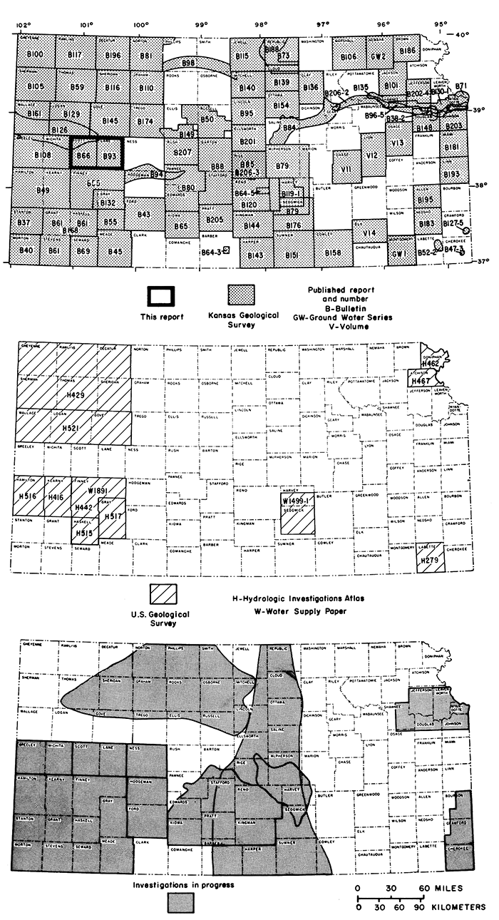
This investigation is a part of a systematic study of the ground-water resources of Kansas that began in 1937. This cooperative program is being conducted by the Kansas Geological Survey and the U.S. Geological Survey with the support of the Division of Water Resources, Kansas State Board of Agriculture, and the Division of Environment, Kansas Department of Health and Environment. The present status of the ground-water investigations in Kansas is shown in figure 17. The numbers on the map refer to Bulletins by the Kansas Geological Survey and to Hydrologic Investigations Atlases and Water Supply Papers by the U.S. Geological Survey.
Figure 17--Index maps showing area discussed in this report, and other areas for which ground-water reports have been published or are in preparation.
Metric Units
For those readers who are familiar with or are interested in the metric system, the English units of measurement given in this report also are given in equivalent metric units (in parentheses) using the following abbreviations and conversion factors:
| English unit | Multiply by | Metric unit |
|---|---|---|
| Length | ||
| inch (in) | 2.54 | centimeter (cm) |
| foot (ft) | .3048 | meter (m) |
| mile (mi) | 1.609 | kilometer (km) |
| nautical mile (nm) | 1.85 | kilometer (km) |
| Area | ||
| square feet (ft2) | 0.0929 | square meter (m2) |
| acre | .4047 | square hectometer (hm2) |
| square mile (mi2) | 2.590 | square kilometer (km2) |
| Volume | ||
| gallon (gal) | 3.785 | liter (L) |
| cubic foot (ft2) | .02832 | cubic meter (m2) |
| acre-foot (acre-ft) | 1.233 X 10⁻³ | cubic hectometer (hm3) |
| Flow | ||
| gallons per minute (gpm) | .06309 | liters per second (L/s) |
| cubic feet per second (f3/s) | .02832 | cubic meters per second (m3/s) |
| Hydraulic conductivity | ||
| feet per day (ft/day) | .3048 | meters per day (m/day) |
| Transmissivity | ||
| square feet per day (f2/day) | .0929 | square meters per day (m2/day) |
| Specific capacity | ||
| gallons per minute per foot (gpm/ft) | .207 | liters per second per meter (L/s)/m |
| Gradient | ||
| feet per mile (ft/mi) | .1894 | meters per kilometer (m/km) |
Prev Page--Unconsolidated Aquifers || Next Page--References
Kansas Geological Survey, Geohydrology
Placed on web June 24, 2013; originally published 1976.
Comments to webadmin@kgs.ku.edu
The URL for this page is http://www.kgs.ku.edu/Publications/Bulletins/IRR1/05_deve.html