![]()
Prev Page—Geology || Next Page—Geological Basis
Geophysical Survey
Instruments, Field Procedure, and Presentation of Data
Introduction
A uniform procedure was employed for the different methods, both in making the field measurements and in compiling and presenting the data.
Station grids and traverses were laid out beforehand in accordance with the general requirements of the geological problems, (see [previous]). These layouts were used for all of the geophysical methods, with changes and additions required as the work progressed.
To aid interpretation, a uniform scale was adopted for plotting the topography, geology, and geophysical anomalies. Insofar as possible, the same scale was used for plotting each series of geophysical data for all of the areas, in order to facilitate comparison of data within areas as well as from area to area. The geophysical data are plotted on maps and profiles in such a way that; (1) the results of the different geophysical methods may be compared and (2) anomalies in each method may be compared to topographic and geologic data.
The corrected geophysical measurements are expressed in the following units:
| Magnetic | gammas |
| Gravity | milligals |
| Natural potential | millivolts |
| Resistivity | ohm-centimeters |
| Geothermal | degrees centigrade |
| Geochemical | relative spectral intensity (arbitrary units) |
On the contour maps the following intervals are employed:
| Topography | 1 foot |
| Geology | 5 feet (except 10 feet in Mullen area) |
| Regional magnetic | 50 gammas |
| Local magnetic | 10 gammas |
| Regional gravity | 0.2 milligals |
| Local gravity | 0.05 milligals |
| Natural potential | 5 millivolts |
| Geothermal | 0.2° C in the Walton area 1.0° C in the Karcher area |
Magnetic Survey
Instruments
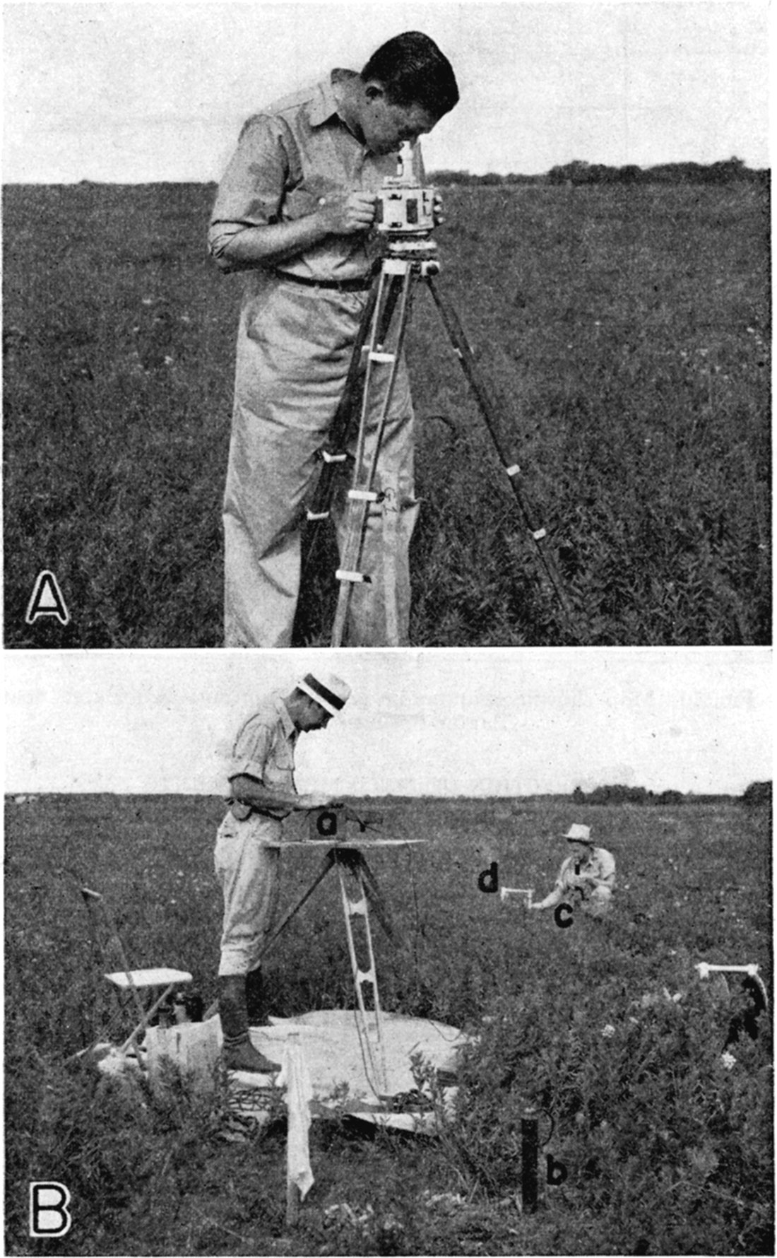
A magnetic vertical field balance of the Askania-Schmidt type was employed for the magnetic studies (pl. 1). This instrument (known also as a vertical magnetometer) measures local variations (anomalies) in vertical magnetic intensity, (Joyce, J. W., 1937).
Plate 1—A. Magnetometer and operator in the field. B. Field set-up for measuring natural earth potentials: a. potentiometer, b. nonpolarizing electrode at base station, c. non polarizing electrode being set at field station, d. reel carrying connecting wire. (After Jakosky, 1940, p. 259.)
Field Procedure
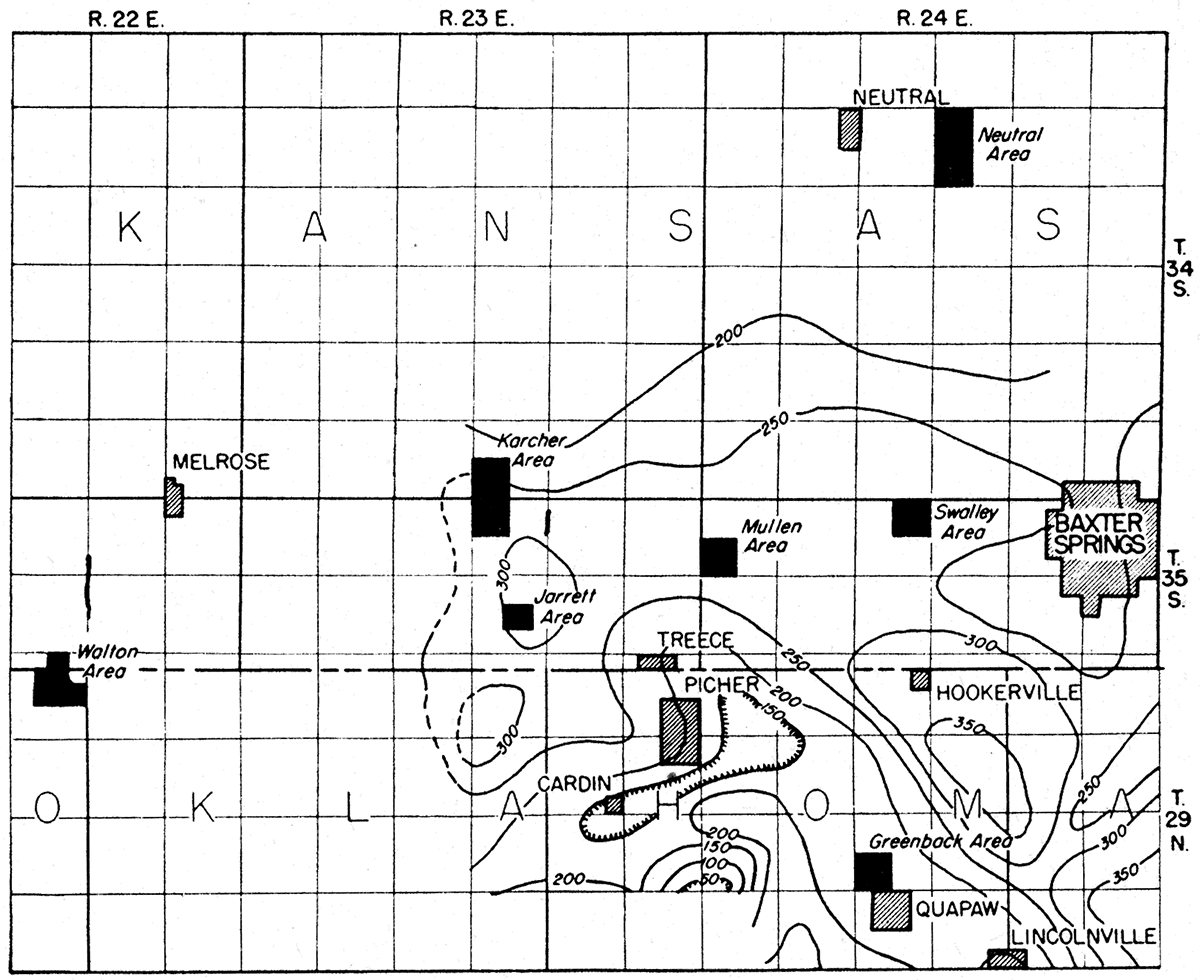
The magnetic work comprised: (1) a regional survey in which readings were taken at intervals of approximately one mile over an area of approximately 75 square miles (fig. 9) and (2) local surveys in which readings were taken at intervals of 50 to 400 feet at grid stations and along traverses in the Neutral, Mullen, Walton, and Karcher areas. Regional and local survey readings were converted to the same datum. The work was conducted by an operator and an assistant.
Figure 9—Isodynamic contour map showing anomalies in vertical intensity of the earth's magnetic field, near Baxter Springs, Kansas.
Correction of Field Measurements
In order to convert the field observations into anomalies of vertical magnetic intensity the corrections listed below were all applied to the magnetic measurements made in the Tri-State area:
- Temperature correction.
- Diurnal correction.
- Latitude correction.
- Longitude correction.
- Base station correction.
- Correction to arbitrary datum.
Temperature Corrections
Changes in temperature affect the magnetic system of the magnetometer in a number of ways that influence its response to variations in strength of the earth's magnetic field. For the instrument used in this survey, the temperature coefficient was 4 gammas per degree centigrade. The scale constant was 1 scale division = 21.0 gammas.
Diurnal Corrections
The approximate diurnal variations were determined by making readings several times during each working day at base stations in the area. Diurnal curves were plotted from the base station readings. Corrections based upon these curves were added to or subtracted from (depending upon their algebraic sign) the readings made at the various stations during the day, so as to eliminate the effect of the diurnal change.
The base station correction was not determined separately from the diurnal correction in this survey. This correction is applied to correct for any change in instrument calibration, especially sudden changes that might be caused by jarring the instrument. No effects of this type were noted during the course of this work.
Latitude and Longitude Corrections
The value of the earth's normal magnetic field varies from place to place over the earth's surface. In surveys extending over distances greater than a mile, it is usually necessary to apply corrections to remove the effect of differences in location (i e., latitude and longitude). Corrections for both latitude and longitude were applied to the Tri-State magnetic readings. For this purpose base lines (lines of zero correction) were assumed as follows: latitude, Kansas-Oklahoma state line; longitude, township line between ranges 24 east and 25 east.
Datum Correction
Absolute values of the magnetic vertical intensity were not computed for this survey. Neither was any particular value of the earth's field chosen as a datum. Instead, an arbitrary datum was employed wherein the lowest reading in the area of the survey (NW cor. sec. 33, T. 29 N., R. 23 E.), was assumed to have zero anomaly. The field readings were then computed in terms of anomalies in gammas above this assumed arbitrary base.
Accuracy of Data
During the course of the magnetic work numerous check readings were made to determine the accuracy of the computed values. Errors in this type of survey are chiefly: (1) errors in field manipulation and observation and (2) errors in applied corrections. As determined experimentally, the sum of these errors probably does not exceed one-half of one scale division (approximately 10 gammas). Variations of more than 10 gammas in any of the areas, therefore, probably represent valid anomalies,
Presentation of Data
The magnetic variations are illustrated in one or both of two ways for the several areas: (1) profiles of anomalies in vertical magnetic intensity (vertical magnetic intensity in gammas plotted against distance in feet) and (2) magnetic isodynamic contours.
Gravity Surveys
Instruments
A Mott-Smith gravity meter was employed in this work. Determination of the relative force of gravity over an area with this instrument consists of "weighing" the same object with very great precision at several stations. The weight of an object at any location on the earth's surface is proportional to the acceleration of gravity, which, in turn, is proportional to the unit mass beneath any given point on the earth's crust. Local variations in the weight of an object are therefore indicative of variations in subsurface mass and, hence, of variations in geologic structure (Jakosky, 1940, pp. 168,180-182).
Field Procedure
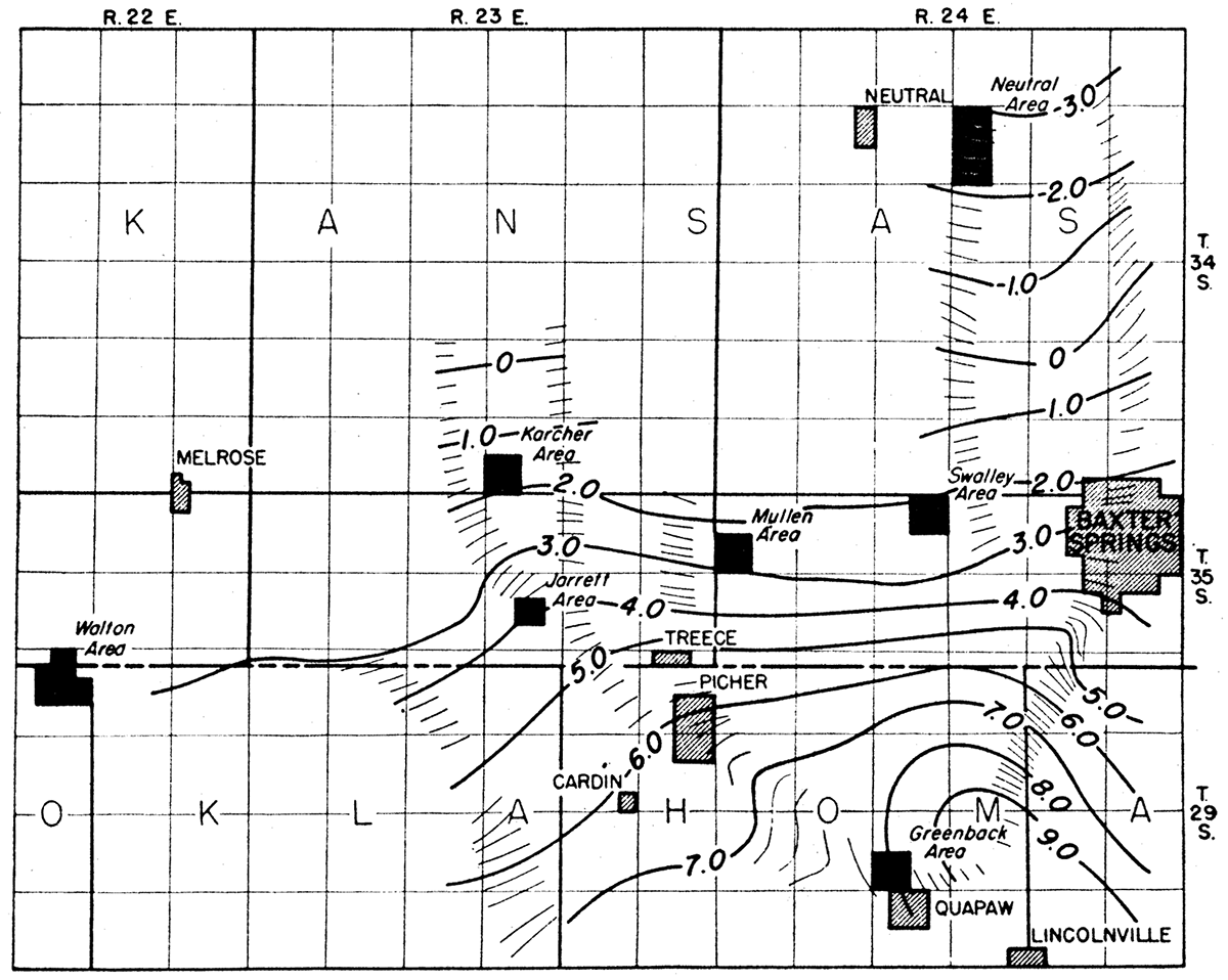
The gravity work comprised: (1) a regional survey in which readings were taken at intervals of approximately one mile, over an area of approximately 60 square miles (fig. 10) and (2) surveys in the 'various local areas in which readings were taken generally at 100 foot intervals along traverses and on grid layouts.
Figure 10—Map showing isanomalic gravity contours in an area near Baxter Springs, Kansas.
In the regional work, the instrument was transported in a closed automobile and the observations were made by setting the instrument on a tripod extending through the floor of the car. For the local areas, the instrument and auxiliary equipment were transported from station to station by hand. This work required two to three men for the gravity observations and a two-man surveying crew for accurately determining the elevations of the gravity stations.
Computation and Correction of Field Measurements
The gravity meter readings are proportional to the changes in acceleration due to gravity. In order to convert these into milligals of acceleration change, it is necessary to apply a number of corrections; It is possible to convert the readings into absolute gravity by tying them in to base stations established by the United States Coast and Geodetic Survey. This was not done for this work since no base has been established nearby. For convenience, an arbitrary base station was set 25 feet east of the northeast corner of the Kansas City Southern Railroad station in Baxter Springs, Kansas. This base was assigned an assumed value of 870 milligals. All readings were tied in to this base, and the computed values shown in this report represent variations from this base value.Calibration of the Instrument
The instrument used in this survey was calibrated by reading it at a series of base stations near Houston, Texas, for which the acceleration of gravity is accurately known, from pendulum observations.
Elevation Correction
In this area the acceleration of gravity decreases at the rate of approximately 0.063 milligals per foot of increase in elevation as determined empirically by measurements made at different levels in mine shafts. Using this factor and the station elevations, the gravity meter readings were reduced to equivalent values at the levels of the base station.
The elevations of the gravity stations were determined to within 0.1 foot by differential leveling. Elevations for several bench marks in the area were obtained from the U. S. Geological Survey in Washington, D. C., and these were used for base stations. A number of closed survey loops were run. The maximum error of closure on any of these was 0.35 feet.
Latitude Correction
The value of the earth's normal gravitational field varies with a change in geographical latitude. The gravity-meter readings, therefore, must be corrected so as to remove the effects of difference in station location. In the Tri-State survey the correction factor was based upon values computed from the International Gravity Formula of 1930. The gravity variation in the area was determined to be 1.2569 milligals per mile.
Regional Gradient
A regional gradient of approximately 1.0 milligal per mile in this area is indicated by the plotted gravity values (fig. 10). It is sometimes desirable to correct for regional gradient in order to more clearly portray local changes. In the present survey, this was necessary only for the Neutral area gravity profile (fig. 16).
Accuracy of Data
Errors in gravity measurements are due chiefly to: (1) reading error due to instrumental variations, (2) errors in calibration, and (3) errors in the elevation and latitude corrections.
The probable reading error as determined from plotting "drift" curves of successive readings at the same station appears to be of the order of 0.03 to 0.05 milligal. It is believed that the calibration for the instrument used in this work is accurate to 0.2 percent. The latitude and elevation were determined with sufficient accuracy to reduce errors from these corrections to less than the reading error. It is believed, therefore, that the sum of these errors probably does not exceed 0.05 milligals. The close agreement between the gravity meter values and the prior torsion balance work in the Jarrett area is interesting and indicates approximately this order of accuracy.
Presentation of Data
The corrected gravity values are plotted as isanomalic contours and as profiles, representing the variation in value above or below the base assumed for the area. The contour interval for all of the local areas is 0.05 milligal, while an interval of 0.2 milligal was used for the regional gravity map.
Natural Potential Survey
Instruments
A Leeds-Northrup potentiometer was used to measure differences in potential associated with natural current flowing in the earth between selected points at the surface. Contact with the ground was made by means of nonpolarizing electrodes consisting of copper rods immersed in saturated solutions of copper sulphate contained in porous cups. Connections between the instrument and the electrodes were made through flexible, rubber-insulated, connecting wire cables wound on hand-operated reels. A photograph of the set-up of instrument and auxiliary equipment is shown in plate 1.
Field Procedure
The purpose of the natural potential measurements was to determine the relative potential and polarity between selected stations in the various areas, so that potential profiles and contours could be plotted therefrom. These stations were located along either traverses (Neutral and Mullen areas) or on a grid work of stations (Walton and Karcher areas).
The instrument was set up at a central station, with one nonpolarizing electrode set in the ground at this station. Other electrodes were then set successively at various stations in the area, and the potential and polarity between the two electrodes observed for each setting. The potentials at the various stations relative to one or more bases in an area thus were determined.
In order to detect potential variations related to changes in intensity and direction of flow of the natural ground currents during any series of measurements, "base" readings were made in several azimuths between points spanning the width of area, or along traverses; as the case required. For each station, the time of reading, potential value, and polarity were recorded.
Computation and Correction of Field Measurements
Computation of the potential readings into values suitable for plotting consisted in: (1) correction for variations indicated by the base station readings (diurnal variations) and (2) reduction of all readings to a common base for each area. In this latter operation the station showing the highest negative polarity in each area was considered to be at zero potential, except in the Walton area where the readings were not reduced to zero base. All computed values, therefore, represent positive potential, relative to a common base, except in the Walton area where both positive and negative potentials are plotted. There is no relationship between the potentials or base values of the separate areas.
Earth potential measurements are subject to a number of errors, the importance of which depend largely upon the smallness of the potentials being measured. In the Tri-State area the potential measured between any two points was seldom more than 20 millivolts, which is a relatively small quantity. Consideration of the possible errors is important.
Three types of influence are mainly responsible for errors in natural potential surveys: (1) variations in electrode contact potential due to variation in soil and moisture conditions around the electrode, and to differences in electrolyte concentration in the electrodes, (2) relatively rapid cyclic variations in earth currents (period usually less than one minute), and (3) earth current fluctuation of slower frequency (variations noted during one day or from day to day).
The first-named error was minimized by employing a uniform procedure for setting electrodes, as well as by careful attention to the non-polarizing electrodes and to the uniformity of the electrolyte. The electrodes were tested occasionally by immersing them in a glass container and measuring the differences in potential. This difference in potential was found to be sometimes as high as 2 millivolts. Although it is not possible to determine the differences in contact potentials due to minor variations at the different electrode set-ups, it is believed that the combined effects enumerated under (1) do not exceed 2 millivolts.
Comparatively rapid earth current fluctuations were noted only occasionally in the area; and, when necessary, the effect of these was minimized by averaging readings over the range of the fluctuation. This error probably does not exceed 2 millivolts.
Variations of a type listed under (3) proved to be serious in this work, especially in the case of the Walton area where the intensity variations were not only especially pronounced during the course of the survey, but were influenced by a somewhat random directional variation for which it was impossible to devise an accurate correction, even from the base station readings made in different azimuths. The reason for these variations is not known.
Accuracy of Data
The accuracy of the natural potential readings is different for the separate areas. A statement of the probable accuracy of the potential values is contained in the discussions under each area. In general; in order of decreasing accuracy, the areas may be listed as follows: Mullen, Neutral, Karcher, Walton.
Presentation of Data
The natural potential values are plotted as equipotential contours and as profiles representing the variation in potential above an arbitrary base assumed for each area. In discussing the results of natural potential work it is customary to use the term "negative center." An area of low· potentials represented by a "depression" contour on the contour map is an area of relative negative potentials, and therefore an area toward which natural current flows, locally, from all directions. Such an area is a negative center. An oxidizing ore body can sometimes be located by detecting the presence of a negative center over the top of the ore body (Jakosky, 1940, pp. 256-266).
Resistivity Survey
Instruments and Measurement Technique
By means of electrical resistivity methods it is possible to secure quantitative electrical data over a controlled range of effective depths. Calculations may be made which will give the average resistivity of the portion of the subsurface included in the measurements.
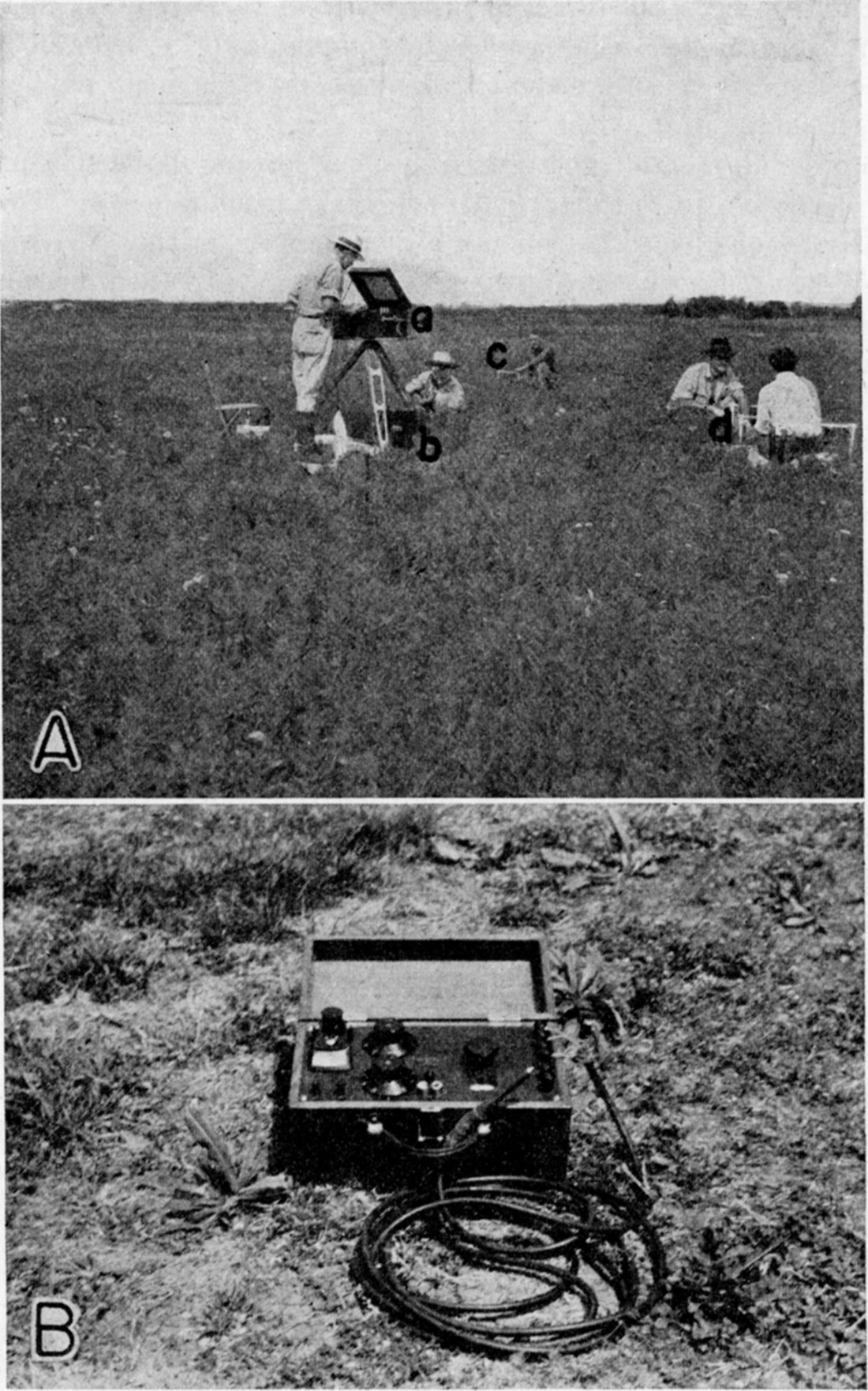
In this work, the electrical ratio instrument was employed. This instrument allows the direct determination of the E:I ratio, thereby simplifying the field measurement technique (Jakosky, 1940, p. 351). Plate 2 shows the instrument and auxiliary equipment set up for measurements in the field.
Plate 2—A. Field set up for measuring earth resistivity: a. electrical ratio instrument, b. battery box, c. reels and electrodes set along line of measurement. B. Thermometer bridge and resistance thermometer.
In order to measure the resistivity of a portion of the subsurface it is necessary to cause current to flow through the earth. This is usually accomplished by passing a measured energizing current between electrodes placed at two selected points and then measuring the potential drop between two or more potential electrodes which are usually placed along a straight line passing through the energizing electrodes. The effective depth of measurement depends upon the configuration and spacing of the various electrodes, and the resistivities of the subsurface strata. From a knowledge of the current, E:I ratio, and the configuration of the electrodes, it is possible to compute the average resistivity of the material included within the zone of measurement. Many types of electrode configurations may be employed.
Two types of resistivity measurements were conducted: (1) lateral investigations and (2) vertical or depth investigations. In the former, ground resistivities are measured over an essentially constant depth range, along a traverse line, for the purpose of detecting horizontal changes across an area. In the latter, resistivities are measured at increments of gradually increasing depth (increasing spread of electrodes) for the purpose of detecting vertical changes (changes in resistivity with depth).
Field Procedure
In this survey four electrodes were spaced equidistant along a straight line, with two potential electrodes inside two energizing electrodes. The spacing between the potential electrodes is therefore equal to one-third of the spacing between the energizing electrodes. This symmetrical arrangement of electrodes facilitates the computations and interpretations and is easily handled in the field. (Wenner, 1916; Gish and Rooney, 1925.)
Power for energization was supplied by a bank of heavy duty "B" type batteries, so assembled that voltages from 22 1/2 volts to 500 volts could be obtained by easy manipulation of a control switch. Spring-steel rods, 2 to 4 feet long, were used as energizing electrodes. The potential electrodes were of the non-polarizing type like those previously described under natural potential procedure. Connections between the various electrodes, power supply, and instrument were made with flexible rubber insulated wire cables wound on hand reels.
Lateral resistivity investigations were conducted along traverses in all areas except the Jarrett area. These lateral studies were of two types: (1) longitudinal traverses and (2) transverse traverses. In the longitudinal traverse, measurements are made as the electrode configuration (spread and spacing remaining constant) is moved along the traverse. The direction of the electrode movement and the direction of measurement, therefore, coincide with the direction of the traverse. In the transverse traverse, measurements are made in a direction at right angles to the direction of the traverse. The electrode configuration (spread and spacing remaining constant) is moved across the area, with the center point of the configuration falling on and moving along the traverse. The electrode spacings used on the various traverses were determined by the depth of investigation required in the different areas. In some of the areas, measurements over two different depth ranges were made along some of the traverses. The locations and directions of the various traverses and the depths and types of measurement conducted along them were governed by geological factors. In general, the traverses cross the significant geological features (mineralized zones or structural trends) at approximately right angles.
Vertical investigations (hereinafter called resistivity depth measurements) were conducted at selected places (stations) in several of the areas, for the purpose of ascertaining their usefulness in the problems of mapping the top of the limestone and securing information to aid interpretation of the lateral measurements. The resistivity work required a personnel of five to seven men.
Computation of Field Measurements
The instrument reading, after making instrumental scale corrections, is the E:I ratio, or resistance of the ground circuit for any particular spacing of the electrodes. This is converted into terms of apparent resistivity from formulae which relate the E:I ratio to factors dependent upon the electrode spacings. In this survey all readings were converted to resistivity in ohm-centimeters.
The resistivity values as computed above are essentially the final values, the only correction subsequently required being a reduction to a common base of values read under variable conditions of temperature, current density, etc. The influence of natural earth currents is eliminated by the use of balancing potentials in the instrument. The chief sources of error in these measurements are: (1) reading errors, (2) error in recorded value due to variation in reading conditions (temperature changes, etc.), and (3) errors in surveying or in setting of electrodes along the lines of measurements. These errors can be minimized by proper technique and care in taking the measurements. The estimated maximum error in this work is about 1 percent of the final computed values.
Factors Influencing Interpretation
The resistivity data in this report are expressed in absolute units. The absolute values are of interest in showing the general range of rock resistivities in the area, but are not useful in interpretation, except in a very general way. For example, it is found that the higher values are found in areas in which the limestone is nearer the surface. Interpretation, with respect to the possible effects of mineralized zones, relief on the limestone surface, brecciated, or cavernous zones, etc., is based primarily upon variations from mean trends along plotted profiles. Resistivity values in the areas range from 6,000 to 20,000 ohm-centimeters over a range of depth extending from the surface to approximately 400 feet.
The penetration factor (ratio of effective depth of measurement to the total spacing of the energizing electrodes) for this area was determined experimentally by making depth measurements at locations where the depths to the limestone were known. For the electrode configuration employed in these tests an approximate value of 0.30 to 0.35 was indicated for the penetration factor.
On some of the resistivity traverses, measurements were made at two different depths. In general, the purpose-of this procedure was to determine the influence of relatively shallow subsurface conditions upon the measurements that were extended to and beyond the depth of the mineralized zones. The computed resistivity values are the weighted averages of aU the resistivity changes present between the surface and the effective depth of measurement. Prominent changes relatively near the surface, therefore, will greatly influence the attempted deeper measurements. The relative influence of shallow and deeper subsurface resistivity changes may be determined from a comparison of the resistivity trends at different depths.
The values of resistivity obtained in these measurements, representing, as they do, weighted values, are more properly termed "apparent" resistivity. A further reason for using the term apparent is the fact that these' values are influenced by the configuration of the electrodes and the direction of the measurements as related to changes in the subsurface. Only in the ideal case of homogeneous, isotropic ground could true values of resistivity be obtained by these measurements.
The effect of the electrode configuration upon the apparent resistivity values is often useful in interpretation. An example of this is the so-called "W" effect, This is a distortion of the normal values along a traverse as the electrode configuration moves across an electrically conductive subsurface zone, and may be explained as follows (fig. 11). Referring to the figure, the positions of the electrodes are shown with reference to a subsurface zone of relatively high conductivity. The energizing electrodes are designated as 1 and 4, and the potential electrodes are 2 and 3 (Jakosky, 1940, p.307).
Figure 11—Anomaly caused by electrically conductive zone crossed by resistivity traverse.
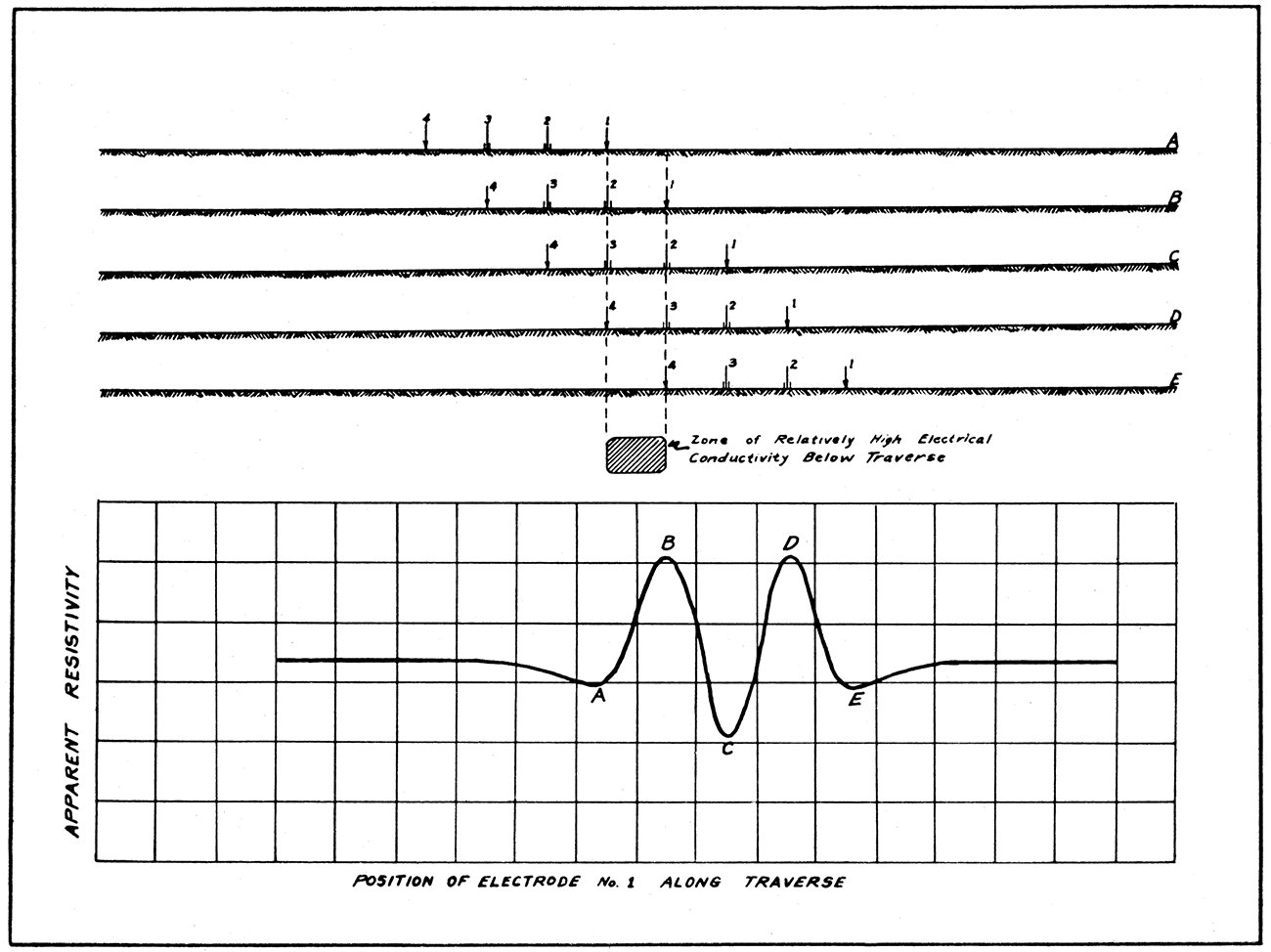
At some distance to the left of the diagram the subsurface is considered to be homogeneous. At this position the current flowing in the ground between electrodes 1 and 4 follows a normal path, and the computed resistivity values are normal. As the electrode configuration approaches the conductive zone, there is a tendency for the current to be concentrated in the better conductor. This causes a diminution in the current density between 2 and 3, resulting in a decreased potential difference. Since the apparent resistivity is proportional to the potential drop between the potential electrodes, this results in a decrease in apparent resistivity, as at A in the lower part of the figure. Now, as the electrode configuration reaches the position shown by B, the potential drop between 1 and 2 becomes less than normal, due to the short circuiting effect of the conductive zone. This causes most of the potential drop to occur between 2 and 3 and, therefore, results in a maximum value of apparent resistivity. When the electrode configuration reaches the position shown by C, the potential difference between 2 and 3 becomes very small since it is measured directly across the conductive zone. For this position the apparent resistivity is a minimum, As the electrode configuration proceeds through positions D and E the effects are similar to the effects noted at B and A, respectively.
It should be noted that the positions of the maximum and minimum resistivity values have a definite relationship to the electrode spacing and the location of the subsurface conductive zone. Recognition of this type of anomaly in the field work is useful, therefore, in determining locations and extents of subsurface conductors.
Presentation of Data
The resistivity traverse data are plotted as profiles of apparent resistivity. These show lateral changes along the lines of the traverses within a selected depth range. The resistivity depth data are plotted as resistivity depth curves which show the variations of resistivity with depth in a restricted zone below the line of measurement.
Geothermal Survey
Instruments and Equipment
The temperature measurements in this area were obtained by the use of Leeds and Northrup resistance thermometers and a Leeds Northrup Semi-Precision Thermometer Bridge (fig. 16). The thermometers consist of resistance elements encased in brass protection tubes, with suitable connecting leads extending from the tubes through heavy rubber conduits. The resistance of the thermometer element varies with changes in temperature. This relationship, having been determined beforehand, is expressed in the form of calibration tables giving the temperature in Fahrenheit and Centigrade degrees for different resistance readings. To determine the temperature at a thermometer station it is necessary only to measure the resistance of the thermometer. This reading is then converted to temperature by consulting the calibration charts.
The thermometer bridge used for the resistance measurements is a double slide-wire Wheatstone bridge designed to measure resistance from 0 to 200 ohms. Measurements accurate to 0.005 ohms (corresponding to ±0.014° C.) can be made easily with this instrument.
Field Procedure
The temperature measurements were taken at selected stations on the traverses and grid layouts. At each temperature station, a hole three feet deep was drilled with a hand-auger, a day or more before the temperature measurements were to be taken. The thermometers were placed in the holes so that the thermometer tube rested firmly against the bottom of the hole or was. pressed into soft soil at the bottom of the hole. After the thermometer was placed in a hole, a cover with a sharp-edged cylindrical flange was fastened securely over the top of the hole.
A uniform reading and thermometer-setting procedure was used so as to minimize the influence of diurnal temperature variations and other extraneous effects. The temperature measurements were made at the same time each morning ordinarily before the atmospheric temperature had started to increase; After completion of the readings, the thermometers were moved to another set of holes in which they were left until the next morning when measurements were again made. Ordinarily the thermometers were left in the holes for at least 16 to 20 hours before reading, so as to insure their reaching equilibrium with the ground temperature.
Although an attempt was made to secure uniform reading conditions, there were many variables that could not be controlled practicably, such as differences in soil and vegetative conditions, variations in topography and surface drainage, and effects of rainfall entering the holes.
Experimental work indicated that three-foot holes are not sufficiently deep to be beyond the range of diurnal variations in this area. However, it was not practicable in this survey to drill deeper holes, and it was found that the practice of making readings at approximately the same time each day sufficiently minimized the effect of the cyclic variation in temperature over a 24-hour period.
Another effect was important. It was noted that, over a period of days, there were fairly uniform increases or decreases in the temperatures measured at base stations. These changes are due apparently to differences in the rate of thermal absorption and radiation by the earth over these periods of time. In order to determine a correction for these variations, a base station was read in each area. The base thermometer was left in the hole throughout the survey of the particular area. Readings of the base station were made each day at the same time, as the other thermometers were read.
Computation and Correction of Field Measurements
Owing to slight fabrication differences, the various thermometers have slightly different temperature coefficients. To determine these differences, the thermometers were calibrated in a water bath over the general range of temperatures measured in the field. One thermometer was used as an arbitrary base. These corrections were applied to the field readings to reduce them to comparable resistance values.
Then, a curve was plotted from the base station readings, showing the variation in ground temperature during the course of the survey. Correction factors derived from this curve were used to reduce all readings in the local area to a common base. The reading, observed at the start of the survey, was arbitrarily taken.
Finally, the resistance readings were converted into terms of temperature in degrees, Centigrade, by reference to the resistance-temperature calibration charts.
Accuracy of Data
The reading accuracy of the thermometer bridge (± 0.014° C.) is an indication of the field measurement accuracy that could be obtained were errors not introduced either by thermometer calibration, by diurnal correction, or by errors inherent in the field procedure. Probably the chief source of error in these measurements is the practical impossibility of setting up the same measurement conditions at different stations, or of duplicating measurement conditions at any one particular station. No attempt was made to segregate or determine the relative effects of different sources of error. Instead, the field procedure was kept as uniform as possible and the probable error. for each area was determined by running a series of check readings.
Reading conditions in the Walton area were somewhat more favorable than in the other areas. The measurements in this area were made after the ground had become saturated with rain water. With but a few exceptions, the readings in this area were made under water. Check readings indicate the probable limit of error to be of the order of 0.2° C.
In the other areas, readings were undoubtedly affected by water seepage from intermittent rainfall, as well as by other local variations related to variations in topography and drainage. These variations were especially prominent in the Karcher area. In the Karcher area the limit of error is believed to be of the order of 0.3° C. to 0.4° C.
Variations in the near-surface conditions are discussed further under the results of the individual areas.
Presentation of Data
The geothermal data are plotted as: (1) isothermal contours and (2) profiles showing the indicated variation in temperature along traverses.
Geochemical Survey
Instruments and Procedure
The samples for geochemical analysis are of two main types: (1) soil samples, taken with a post-hole auger at a depth of three feet, and (2) drill hole samples, taken at more or less regular intervals from selected exploratory drill holes in Kansas and Oklahoma. There are two types of drill hole samples: (1) samples from the Cherokee shale and (2) samples from the Mississippian limestone.
All samples were given identical preparation. First, they were crushed so that they would pass through a Jones sample splitter. Next, a 20 gram sample was ground to minus 60 mesh. The sample was then placed in a manila envelope and labeled. Subsequently, before making the analysis, the contents of the envelope were poured out on a clean sheet of wrapping paper and mixed by lifting corners of the paper and rolling the sample. A quarter of the sample was cut out and mixed to provide the sample for analysis. The weight of the sample used for analysis was about 0.1 gram.
An Applied Research Laboratory grating spectrograph was used for the analyses. The wave length range employed was about 2,400 to 4,550 angstroms (which includes the most useful portions of the visible and ultra-violet spectra).
Two graphite rods, five-sixteenths of an inch in diameter and 3 inches long, were used for electrodes. Two holes were drilled one-fourth inch deep in the top of the lower electrode as a container for the sample. The upper electrode was sharpened in a pencil sharpener and the point flattened off with a carbon steel file.
The electrodes were spaced 5.5 mm. apart and a portion of the sample placed in the holes drilled in the lower electrode. The exposure was made by starting an electric arc across the gap and letting it run for one minute. The potential across the gap was 115 volts and the current flow was about 8 amperes.
Eastman number 10 negative 35 mm. film was used for the spectrograms, eight samples being run on a single strip of film 18 inches long. The spectrograms were read by projecting them onto a screen and comparing the lines on the spectrogram with a series of cards indicating the position of the significant lines. The intensities of those lines which were present were estimated by visual inspection using an arbitrary scale of spectral intensity. Increasing numbers on this arbitrary scale indicate increasing spectral intensity. The numbers presented on the accompanying geochemical maps and profiles indicate these arbitrary spectral intensities.
The set of master cards used in locating the significant lines was prepared by Dr. J. H. McMillen, of the Department of Physics at Kansas State College. The scale of these cards is, approximately: 0.6 centimeter equals one angstrom, a scale which makes it possible to differentiate between lines only 0.2 angstrom apart. Table No. 1 gives a list of lines used:
Table 1—List of elements and spectral lines used in the spectrographic analyses.
| Wave length, Å | Element | Wave length, Å | Element | |
|---|---|---|---|---|
| 2,496.8 | Boron* | 3,261.59 | Titanium | |
| 2,536.52 | Mercury * | 3,273.96 | Copper * | |
| 2,652.48 | Aluminum | 3,280.67 | Silver * | |
| 2,741.2 | Lithium | 3,282.33 | Zinc or Titanium | |
| 2,801.08 | Manganese | 3,302.94 | Sodium * | |
| 2,802.71 | Magnesium | 3,345.02 | Zinc* | |
| 2,833.07 | Lead * | 3,345.51 | Zinc | |
| 2,839.99 | Tin* | 3,345.91 | Zinc | |
| 2,860.46 | Arsenic * | 3,391.96 | Zirconium | |
| 2,877.92 | Antimony * | 3,414.77 | Nickel* | |
| 2,897.98 | Bismuth * | 3,446.37 | Potassium | |
| 2,905.9 | Gold | 3,451.4 | Boron | |
| 2,908.81 | Vanadium | 3,453.51 | Cobalt" | |
| 2,943.70 | Gallium * | 4,008.76 | Tungsten * | |
| 3,039.08 | Germanium * | 4,034.45 | Manganese * | |
| 3,096.9 | Magnesium | 4,047.2 | Potassium | |
| 3,122.79 | Gold | 4,077.71 | Strontium" | |
| 3,132.6 | Molybdenum | 4,254.34 | Chromium * | |
| 3,175.04 | Tin | 4,294.62 | Tungsten | |
| 3,256.08 | Indium or Manganese | 4,358.34 | Mercury | |
| 3,261.05 | Cadmium* | 4,554.04 | Barium* | |
| * Most sensitive line in this range. | ||||
Several of these lines were not found on any of the spectrograms . and others are of doubtful value because of the presence of interfering lines. A list of the interfering lines and a discussion of each element is given on pages 55-60. A 35 mm projector was used for projecting the spectrograms. An assistant ran the projector and recorded the readings.
Spectrograms which are similar can be read. very rapidly by this procedure. The soil sample spectrograms proved easiest to read, with the shale sample spectrograms second. Spectrograms for the limestone and chert samples were much more difficult, requiring about a 3-fold longer reading time per sample. This is due chiefly to the absence of many of the iron and titanium lines which were used as guides in locating the significant lines.
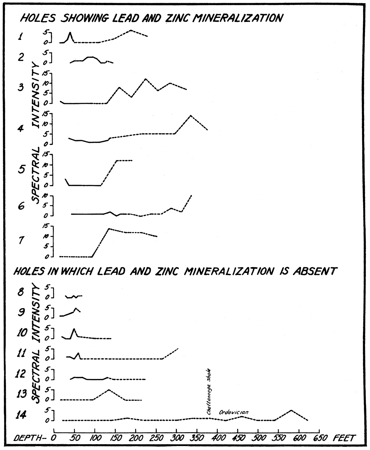
Figure 15—Vertical distribution of zinc in drill holes. For location of drill holes see table 13, p. 86.
Discussion of Elements
The numbers following the name of the elements are the wave lengths of the lines of that element for which readings of intensity were taken.
Boron, 2,496.8 and 3,451.4 Å
The first of these lines is very difficult to read because of the bands in the background. Almost no variation in intensity was detected in the soil samples but there is some variation in the drill hole samples. The line at 3,451.4 Å was not detected in any of the sample analyses. There are no coincident lines, but the 2,496.54 Å iron line is very near the first-named Boron line.
Mercury, 2,536.52 and 4,358.34 Å
The first of these lines is about ten times as strong as the second, but it was not usable because of interference by band spectra. An indistinct line was present at a wave length of 4,358.34 Å, but it is doubtful if this indicates the presence of mercury.
Aluminum, 2,652.48 Å
This line was chosen because the more sensitive lines were too strong. Small differences in intensity cannot be determined on strong lines. There are no coincident lines which could cause reading trouble, but there are bands which make difficult the reading of the very low intensities.
Large differences in intensity were found when using this line, but these differences may not indicate variations in the aluminum content. Variations on repeating the same sample are often as great as the variations between samples.
Lithium, 2,741.20 Å
This line is easily identified but does not vary greatly in intensity. It is present on most of the spectrograms.
Manganese, 2,801.08 and 4,034.45 Å
Both of these lines are distinct and there are no interfering or coincident lines. Manganese is not present in the carbon electrodes. Both lines show considerable variations in intensity readings for different samples and give consistent readings in the same sample. The 4,034.45 Å line is more sensitive than the 2,801.08 Å line.
Magnesium,2,802.71 and 3,096.9 Å
The 2,802.71 Å line is a heavy line and does not show valid differences in intensity on any of the soil or shale sample spectrograms. For this reason the 3,096.9 Å line was used for the drill hole samples. The 3,096.9 Å line is fuzzy and indistinct but shows considerable variation.
The 2,802.71 Å line shows up in analyses of the electrodes, but the 3,096.9 Å line does not.
Lead, 2,833.07 Å
Lead was detected in all of the shale samples and in most of the soil samples. The intensity of this line does not vary much, except in the mineralized zones in the limestone. There are no coincident lines.
Tin, 2,839.99 and 3,175.04 Å
There are interfering lines of chromium at 2,840.02 Å, aluminum at 2,840.11 Å, and tellurium at 3,175.13 Å. There is also a thick, fuzzy line or band at about 2,840 Å. The tellurium line at 3,175.13 Å was used originally to identify tellurium, but this can not be differentiated from 3,175.04 Å. Identification of tin is not certain unless both lines are present.
Arsenic, 2,860.46 Å
This is the most sensitive line available and there are no coincident lines. This line was not present on any of the spectrograms. The absence of the line does not mean that arsenic was absent in the sample; it merely indicates that arsenic was not present in sufficient quantities to be detected under the conditions of the procedure employed.
Antimony, 2,877.92 Å
This line is very near a heavy "ghost" line which sometimes causes difficulty in identification. Antimony was detected in only one sample.
Bismuth, 2,897.98 Å
This line occurs in a very clear portion of the spectrum and there is no danger of coincidence except from platinum at 2,897.88 Å. A trace of bismuth was detected in only a very few samples.
Gold, 3,122.79 and 2,905.90 Å
There are lines near by which might possibly be confused with gold: titanium at 3,123.07 Å, vanadium at 2,906.13 Å, chromium at 2,905.5 Å, and platinum at 2,905.90 Å. Gold was not detected in any of the samples.
Vanadium, 2,908.81 Å
The only possibility of coincidence is with chromium, at 2,909.06 Å. Vanadium is present as an impurity in the electrodes and is present in most of the samples. The intensity of this line is seldom over 5.
Gallium, 2,943.70 Å
Gallium does not occur in the electrodes and there are no coincident lines. This line is much more prominent in the soil and shale samples than in the limestone and chert samples.
Germanium, 3,039.08 Å
Germanium does not occur in the electrodes and there are no coincident lines. Germanium was detected only in a few of the ore samples.
Molybdenum, 3,132.06 Å
Molybdenum does not occur in the electrodes and there are no coincident lines. Molybdenum was indicated in some of the samples.
Indium, 3,256.08 Å
An interfering line of manganese at 3,256.14 Å renders this identification doubtful. All samples in which this line was identified were high in manganese.
Cadmium, 3,261.05 Å
This is a sensitive line with no seriously interfering lines. Cadmium is not present in any of the soil or shale samples but was found frequently in the limestone samples obtained near the ore horizons.
Titanium, 3,261.59 Å
This is not the most sensitive line for titanium, but it was utilized because the more; sensitive lines are too heavy. Titanium occurs in the electrodes and in most of the samples.
Zinc, 3,282.33 Å, 3,345.02 Å, 3,345.51 Å, 3,345.91 Å
There is a titanium line at 3,282.33 Å which makes the zinc line at 3,282.33 Å useless for samples of low zinc counterfeit. The 3,282.33 Å zinc and titanium line occurs in most of the soil samples, but cannot be used for identification of zinc. There are three zinc lines between the wave lengths 3,345 Å and 3,346 Å. The 3,345.02 Å line is the most sensitive and the 3,345.91 Å is the least sensitive. The first of these lines occurs in a very few of the soil samples. All three are prominent in the ore samples. The possible interfering lines are zirconium 3,344.7 Å, cerium 3,344.76 Å, and molybdenum 3,344.75 Å.
Copper, 3,273.96 Å
This is the most sensitive copper line. There are no interfering lines. Very little variation in intensity was noted in some of the limestone samples. Copper occurs in the electrodes and in all of the samples.
Silver, 3,280.67 Å
This is the most sensitive silver line and there are no coincident lines. Silver is present in many of the samples but does not give consistent quantitative results.
Sodium, 3,302.94 Å
Sodium occurs in almost all the soil and shale samples and in most of the limestone samples. There is a zinc line at this wave length which makes this line useless for determinations on the ore samples. There is another zinc line at 3,302.59 Å which is slightly more sensitive; and, if it is absent, then the 3,302.94 Å zinc line will not cause trouble.
Zirconium, 3,391.96 Å
Zirconium occurs in most of the soil samples, but it varies as much when a sample is repeated several times as it does between different samples. For this reason zirconium could not be used in this study.
Nickel, 3,414.77 Å
This is the most sensitive nickel line and there are no coincident lines. Nickel is present in most of the samples.
Cobalt, 3,453.51 Å
This is a very useful line because it is in a clear portion of the spectrum, shows considerable variation on different samples, and gives consistent readings on the same sample. There is a chromium line at 3,453.33 Å, but this is far enough away to prevent mistaking it for the cobalt line. Cobalt occurs in most of the samples and ranges in intensity from 0 to 7.
Tungsten, 4,008.76 and 4,294.62 Å
The line at 4,008.76 Å is very difficult. to read because of the bands. There is a titanium line at 4,008.93 Å. The 4,294.62 Å line is less sensitive but is in a clear portion of the spectrum. Tungsten was not identified in any of the samples.
Potassium, 4,047.2 Å
An attempt was made to use the potassium line at 3,446.37 Å, but the 3,446.4 Å cobalt line interfered. Therefore, the 4,047.2 Å potassium line was used, although it is subject to interference by band spectra.
Strontium, 4,077.71 Å
This is a heavy, wedge-shaped line which shows up through the bands. Because of its irregular shape it is impossible to read this line accurately. Strontium is present in aU of the samples and also in the electrodes.
Chromium, 4,254.34 Å
This is the most sensitive chromium line and there are no coincident lines. Chromium shows very little variation in the soil and shale samples. Larger intensity variations were found in the limestone samples. The. presence of chromium (in very low intensities) is indicated on a few of the electrode spectrograms.
Barium, 4,554.04 Å
Barium has a wedge-shaped, heavy line which is impossible to read accurately. Barium is present in all of the samples and is prominent in the electrode spectrograms.
Relation Between Spectral Intensity and Sample Composition
The spectrograph is, primarily, an instrument for the qualitative detection of minute quantities of the various elements. Since variations in the amount of an element present in a given sample, however, cause variations in the intensity of the spectral lines of that element, it is possible to use the spectrograph for quantitative analyses. The rate of increase or decrease of spectral intensity, however, is not a direct function of the rate of increase or decrease in quantitative content of an element within a sample. Therefore, in order to make exact quantitative spectrographic analyses, it is necessary to plot variations in spectral intensity as a function of known variations in elemental composition. To make such exact quantitative spectrographic analyses requires much time and expense. Such relationships between spectral intensity and elemental composition, moreover, are valid only as long as the particular element occurs in material of, essentially the same composition. Since, for this work, it was necessary to make a large number of quantitative determinations and since a number of rock types were analyzed, it was necessary to use, instead, a method of semi-quantitative analyses. The intensities of selected spectral lines, thus, were estimated visually by comparison with an arbitrary standard; and the estimated spectral intensities were given arbitrary values. It is these arbitrary values of spectral intensity which have been used in this report.
These arbitrary values indicate only the relative amounts of one element in several samples. There is no direct relationship between the arbitrary values assigned to various elements, nor is there any direct relationship between variations in quantitative content of an element and variations in the arbitrary spectral intensity values. A cobalt reading of 4, for example, indicates more cobalt than a cobalt reading of 2 and less cobalt than a cobalt reading of 8. It does not, however, mean that the sample having a spectral intensity of 4 has twice as much cobalt as the sample showing a spectral intensity of 2, nor half as much as a sample showing a spectral intensity of 8. Nor does a spectral intensity reading of 2 for both cobalt and vanadium indicate that the same amounts of both elements are present in the sample. It means only that all cobalt readings of 2 indicate approximately the same amount of cobalt in the sample (within limits to be noted).
Occasionally, two spectral lines were read for the same element. In such cases, it is to be noted that intensity values may be different for the two lines. Manganese, for example, is an element for which two different lines were read. The A-10 sample on the Swalley area gives an intensity reading of 10 for the 2,801.08 Å line and a reading of 15 for the 4,034.45 Å line. The E-7 sample on the same area reads 5 for both lines. These results show that the 4,034.45 Å line is more sensitive to changes in the amount of manganese present than is the 2,801.08 Å line.
Accuracy of Data
Sources of Analytical Error
There are many possible sources of error in the spectrographic method used in this work. The important sources of error are listed below in approximately the order of their importance:
- Errors due to variations in arcing conditions.
- Errors due to variations in visual determination of spectral intensity.
- Errors due to the presence of impurities in the electrodes.
- Errors due to interfering lines.
- Errors due to contamination of sample.
- Errors due to sampling.
- Errors due to slight variations in method of developing spectrograms.
- Errors due to slight variations in exposure time.
Errors due to variations in arcing conditions—The electric arc, which is the cause of volatilization producing the spectrum, shifts from one side of the electrode to the other. This erratic movement causes a difference in the amount of light received by the spectrograph and consequently a difference in spectral intensity on the spectrograms. Another factor is that the position of the electrodes cannot be kept exactly the same for all exposures. There are also minor fluctuations in current and voltage.
The magnitude of the error due to variations in arcing conditions is difficult to determine because of other possible sources of error present at the same time.
The probable magnitude of this error is indicated in the readings tabulated in table No. 2, which are from samples which were arced four times on the same film. Comparison of samples run on the same film eliminated much of the reading error; and, thus, the differences obtained are due largely either to variation in arcing conditions or to the sampling procedure.
Table 2—Comparison of spectral intensity values for three samples which were arced four times.
| Al | Mn | Pb | V | Ga | Ti | Cu | Ag | Na | Zr | Ni | Co | Mn | |
|---|---|---|---|---|---|---|---|---|---|---|---|---|---|
| WD 4 | 5 | 5 | 1 | 2 | 1 | 5 | 5 | 2 | 4 | 2 | 1 | 1 | 4 |
| WD 4 | 2 | 4 | 1 | 1 | 1 | 4 | 6 | 0 | 3 | 0 | 1 | 1 | 5 |
| WD 4 | 4 | 4 | 1 | 2 | 1 | 5 | 6 | 0 | 3 | 0 | 1 | 0 | 3 |
| WD 4 | 7 | 5 | 1 | 1 | 1 | 5 | 5 | 0 | 4 | 2 | 2 | 0 | 4 |
| WA 16 | 3 | 5 | 1 | 2 | 2 | 5 | 7 | 1 | 5 | 1 | 2 | 0 | 4 |
| WA 16 | 4 | 5 | 1 | 2 | 2 | 5 | 6 | 1 | 4 | 1 | 2 | 0 | 4 |
| WA 16 | 5 | 4 | 0 | 0 | 0 | 3 | 6 | 0 | 2 | 0 | 1 | 0 | 3 |
| WA 16 | 4 | 5 | 1 | 1 | 1 | 5 | 6 | 0 | 5 | 0 | 2 | 1 | 4 |
| KF 4 | 9 | 8 | 2 | 4 | 3 | 5 | 6 | 0 | 4 | 3 | 4 | 4 | 10 |
| KF 4 | 4 | 8 | 2 | 4 | 2 | 5 | 6 | 1 | 4 | 1 | 4 | 4 | 10 |
| KF 4 | 6 | 8 | 2 | 4 | 2 | 5 | 6 | 0 | 4 | 0 | 4 | 4 | 10 |
| KF 4 | 4 | 8 | 2 | 4 | 3 | 5 | 6 | 0 | 5 | 1 | 4 | 4 | 9 |
The error due to variations in arcing conditions seldom exceeds an intensity of 1, except for aluminum, silver, and zirconium. Because of the large intensity variations for these three elements, their relative concentrations in the various samples could not be determined accurately by the methods employed in this analysis. The variation shown by the third spectrogram of WA 16 is the extreme example of errors due to variations in arcing conditions.
Errors due to variations in uisual. determination of spectral intensity—The ability of a person to uniformly estimate the intensities of lines on a spectrogram is a result of his personal temperament and various other factors involved in the reading conditions. The limitation may introduce errors of considerable importance. A range of intensities from 1 to 20 was used, except in a very few cases where higher intensities were indicated. A line which was barely detectable was assigned an intensity of 1, a distinct black line, 5, and a slightly thickened, heavy black line, 10. Above 10, distinctions were made on the basis of the thickness of the line.
For most of the elements the error in estimating the spectral intensities is as great as the arcing error. This error is especially significant when readings taken a week or more apart are compared. The accuracy of the intensity readings depends upon spectrogram background, the distinctness of the line, and the uniformity of the line. Consistent readings are not possible for lines such as the barium and strontium lines, which are thick, but wedge out.
The magnitude of the reading error can be determined by reading the same spectrogram on different dates. Table No. 3 is a compilation of the results of check readings of 24 samples from the Swalley area, read 10 days apart.Table 3—Spectral intensity variations in samples read ten days apart.
| (a) Duplicate reading (Percent) |
(b) Variation of one (Percent) |
(c) Variation of two (Percent) |
|
|---|---|---|---|
| Mn | 54 | 29 | 19 |
| Pb | 83 | 17 | |
| V | 50 | 50 | |
| Ga | 92 | 8 | |
| Mo | 75 | 25 | |
| Ti | 67 | 33 | |
| Cu | 63 | 33 | 4 |
| Ag | 79 | 21 | |
| Na | 42 | 58 | |
| Zr | 75 | 25 | |
| Ni | 75 | 25 | |
| K | 67 | 33 | |
| Co | 50 | 50 | |
| Mn | 25 | 58 | 17 |
| Ba | 54 | 38 | 8 |
The data in table No. 3 shows that the error in reading intensities is seldom greater than an intensity of one. The actual reading error on a given area is probably less than is indicated by the above table, because, with the exception of the Walton area, all samples from each area were read in a single day.
The reading error could be eliminated by reading the lines on a photo-electric densitometer. This method is very accurate, but it would not be practical for so many elements because of the greatly increased time required for the readings. If one or two lines of special significance were to be found, it might be practical to read them by this method.
Errors due to impurities in the electrodes—Ordinary spectrographic carbons of the type used for this study contain appreciable amounts of iron, silicon, magnesium, titanium, copper, calcium, aluminum, vanadium, boron, strontium, barium, and chromium. The presence of any of these elements in the spectrogram is not conclusive proof that it is present in the sample unless the intensity in the sample is substantially greater than the corresponding line from an electrode test.
The effect of the impurities in the electrodes is largely masked when a sample is run. For example, several samples show an absence of titanium and vanadium although both of these elements were present in electrode tests taken at the same time. Strontium and barium show up stronger in the electrode tests than they do in most of the samples.
Electrodes can be obtained which are practically free of impurities, but only at considerable greater cost. There are methods of removing the impurities by leaching with acids or heating to high temperatures. No attempt was made in this study, however, to eliminate the error due to impurities in the electrodes.
Errors due to interfering lines—One of the main advantages of the grating spectrograph (here used) over the prism type is that the former has a linear scale. After the wave lengths of a few prominent lines are determined, it is relatively simple to locate the position that a line of a given wave length would occupy.
Thirty-one elements and 42 lines were considered in the analyses here presented. Many of these lines were never present and some were not usable because of interfering or coincident lines. Gold, arsenic, and tungsten were not identified in any of the samples; and the identification of bismuth, antimony, tellurium, indium, and mercury is questionable.
Enlarging the spectrogram by projection made it possible to differentiate between lines 0.2 of an angstrom apart, provided that neither line was very heavy. Any line which is less than 0.2 of an angstrom from a line which is being used for identification might make identification difficult. Heavy lines may cause trouble even when 0.5 Å apart.
In this study several lines which were chosen originally had to be discarded because of interfering lines. The zinc line with a wave length of 3,282.33 Å could not be used in the soil sample analyses because of a titanium line at the same wave length. A tellurium line with a wavelength of 3,175.13 Å was not usable because of the presence of a tin line with a wave length of 3,175.04 Å. This line was used to confirm the presence of tin, because the tin line at 2,839.99 Å has interfering lines of aluminum and chromium. The indium line at 3,256.08 Å could not be used because of a manganese line at 3,256.14 Å. A check was made of the samples in which indium had been identified; and, in all cases, those samples were high in manganese. A discussion of the possible interfering lines is given in the previous discussion of each element ([previous]).
Errors due to contamination of samples—Contamination of the samples is an ever-present danger when dealing with metals which are present in such small quantities. Although many precautions were taken against such contamination, there is no doubt that small errors were introduced.
Drill hole samples are always subject to contamination from overlying formations and metals present in the drill bit or sample containers. The drillers poured the drill hole samples into small pits where they remained until they were collected several days later.
Most of the sources of contamination apply only to the drill hole samples. The soil samples are more nearly free from contamination.
Errors due to sampling—No checks were run on the sampling procedure (see [previous]). It would be difficult to differentiate such errore from the error due to variations in arcing conditions.
Errors due to variations in method of developing spectrograms—Any changes in temperature, concentration of developer, or time of development would cause variations in the intensity of the lines on the spectrograms. All of these factors were held nearly constant in this study, and it is not likely that any appreciable errors were introduced by the developing procedure.
Errors due to variations in exposure time—The exposure was made by allowing the electric arc to run for 60 seconds. It was not exceptional for the arc to go out one or more times, which made accurate timing difficult. This variation in timing seldom exceeded 5 seconds. Two test readings to 90 seconds show only slight differences from those of 60 seconds. Slight differences in exposure time do not seem to make any significant differences in the results.
Validity of Readings
In view of the many possible sources of error one might wonder if any results could be considered valid. By taking several readings of the same sample, however, the maximum variation can be determined. This maximum variation is the sum total of all the errors except those due to contamination and mis-identification. Any differences between two samples which exceed the variations in repeated readings of the same samples can be considered valid differences in chemical composition.
Validity of soil samples—A compilation of the results of 73 readings taken on 14 samples from the various areas is given in Table No. 4.
Table 4—Results of check readings on soil samples
| Duplicate readings |
Vary by one unit |
Vary by two units |
||||
|---|---|---|---|---|---|---|
| Manganese | 53 | 72.6% | 19 | 26.0% | 1 | 1.4% |
| Lead | 55 | 75.2 | 17 | 23.4 | 1 | 1.4 |
| Vanadium | 53 | 72.2 | 17 | 23.4 | 3 | 4.0 |
| Gallium | 52 | 71.2 | 17 | 23.4 | 3 | 4.0 |
| Molybdenum | 59 | 80.8 | 13 | 17.8 | 1 | 1.4 |
| Titanium | 58 | 79.4 | 14 | 19.2 | 1 | 1.4 |
| Nickel | 56 | 76.7 | 16 | 23.0 | 1 | 1.4 |
| Cobalt | 52 | 71.2 | 20 | 27.4 | 1 | 1.4 |
In this list of eight selected elements nearly 75 percent of the readings were duplicated when repeated. Only 2.5 percent of the readings varied more than 1 unit from the standard reading. The above table shows that a difference in line intensity of 2 units for any of the selected elements almost always represents a valid difference in the amount of that element present in the sample. The few exceptions to this rule can practically be eliminated by questioning the validity of single station anomalies.
In a few cases a difference of 2 was not considered valid for vanadium and gallium. This is true on the Swalley, Walton, and Karcher areas.
Out of 31 elements for which readings were taken, all but nine were eliminated from consideration in the soil samples.
Elements which do not occur or occur only rarely in the soil samples could not be used. These elements are: gold, tin, antimony, bismuth, germanium, cadmium, and tungsten.
There are a number of elements which were eliminated because the arcing error exceeded the differences between samples. These elements are: aluminum, zirconium, sodium, and silver.
Elements which are prominent in the electrodes were eliminated. These include magnesium, copper, strontium, and barium.
Boron, lithium, copper, and chromium seldon vary in intensity by more than one, so they were eliminated from consideration.
Elements for which there are coincident lines are: zinc, potassium, teUurium, and indium. The identification of mercury is uncertain.
Only manganese, lead, vanadium, gallium, titanium, molybdenum, nickel, and cobalt, therefore, remain to be considered in the discussion of results.
The following tables are a compilation of the total variation for each area compared with the analytical variation within a given sample. For example the readings for manganese on the Swalley area range from 4 to 10 and the analytical error in determination of individual samples is only one. This indicates that a number of valid differences in manganese content can be plotted for this area.
Table 5—Table comparing total variation of spectral intensities with analytical errors for each element—Mullen area.
| Element | Number of samples having line intensity of... | Sample number |
||||||||||
|---|---|---|---|---|---|---|---|---|---|---|---|---|
| 0 | 1 | 2 | 3 | 4 | 5 | 6 | 7 | 8 | 9 | 10 | ||
| Mn | 14 | 11 | 8 | 3 | 3 | Entire area | ||||||
| 2 | 1 | II 6 | ||||||||||
| 1 | 2 | II 14 | ||||||||||
| Pb | 3 | 34 | 2 | Entire area | ||||||||
| 3 | II 6 | |||||||||||
| 3 | II 14 | |||||||||||
| V | 3 | 25 | 11 | Entire area | ||||||||
| 2 | 1 | II 6 | ||||||||||
| 2 | 1 | II 14 | ||||||||||
| Ga | 1 | 9 | 20 | 8 | 1 | Entire area | ||||||
| 3 | II 6 | |||||||||||
| 2 | 1 | II 14 | ||||||||||
| Mo | 3 | 33 | 3 | Entire area | ||||||||
| 3 | II 6 | |||||||||||
| 3 | II 14 | |||||||||||
| Ti | 26 | 13 | Entire area | |||||||||
| 3 | II 6 | |||||||||||
| 3 | II 14 | |||||||||||
| Ni | 7 | 25 | 7 | Entire area | ||||||||
| 3 | II 6 | |||||||||||
| 3 | II 14 | |||||||||||
| Co | 13 | 14 | 6 | 5 | 1 | Entire area | ||||||
| 1 | 2 | II 6 | ||||||||||
| 3 | II 14 | |||||||||||
Table 6—Table comparing total variation of spectral intensities with analytical errors for each element—Walton area.
| Element | Number of samples having line intensity of... | Sample number |
||||||||||
|---|---|---|---|---|---|---|---|---|---|---|---|---|
| 0 | 1 | 2 | 3 | 4 | 5 | 6 | 7 | 8 | 9 | 10 | ||
| Mn | 2 | 42 | 102 | 3 | Entire area | |||||||
| 2 | 3 | WD 4 | ||||||||||
| 1 | 3 | 1 | WM 4 | |||||||||
| 2 | 3 | WH 13 | ||||||||||
| 1 | 4 | WA 16 | ||||||||||
| Pb | 3 | 132 | 15 | Entire area | ||||||||
| 5 | WD 4 | |||||||||||
| 2 | 3 | WM 4 | ||||||||||
| 4 | 1 | WH 13 | ||||||||||
| 1 | 4 | WA 16 | ||||||||||
| V | 4 | 74 | 69 | 4 | Entire area | |||||||
| 3 | 2 | WD 4 | ||||||||||
| 2 | 2 | I | WM 4 | |||||||||
| 2 | 3 | WH 13 | ||||||||||
| 1 | 4 | WA 16 | ||||||||||
| Ga | 25 | 101 | 7 | Entire area | ||||||||
| 5 | WD 4 | |||||||||||
| 1 | 4 | WM 4 | ||||||||||
| 1 | 4 | WH 13 | ||||||||||
| 1 | 1 | 3 | WA 16 | |||||||||
| Mo | 147 | 4 | Entire area | |||||||||
| 5 | WD 4 | |||||||||||
| 5 | WM 4 | |||||||||||
| 5 | WH 13 | |||||||||||
| 5 | WA 16 | |||||||||||
| Ti | 1 | 26 | 121 | 3 | Entire area | |||||||
| 2 | 3 | WD 4 | ||||||||||
| 1 | 2 | 2 | WM 4 | |||||||||
| 1 | 4 | WH 13 | ||||||||||
| 1 | 4 | WA 16 | ||||||||||
| Ni | 9 | 122 | 20 | Entire area | ||||||||
| 4 | 1 | WD 4 | ||||||||||
| 1 | 3 | 1 | WM 4 | |||||||||
| 3 | 2 | WH 13 | ||||||||||
| 1 | 4 | WA 16 | ||||||||||
| Co | 56 | 88 | 7 | Entire area | ||||||||
| 3 | 2 | WD 4 | ||||||||||
| 4 | 1 | WM 4 | ||||||||||
| 4 | 1 | WH 13 | ||||||||||
| 3 | 2 | WA 16 | ||||||||||
Table 7—Table comparing total variation of spectral intensities with analytical errors for each element—Karcher area.
| Element | Number of samples having line intensity of... | Sample number |
||||||||||
|---|---|---|---|---|---|---|---|---|---|---|---|---|
| 0 | 1 | 2 | 3 | 4 | 5 | 6 | 7 | 8 | 9 | 10 | ||
| Mn | 1 | 26 | 24 | 20 | 18 | 2 | Entire area | |||||
| 4 | 1 | KG 6 | ||||||||||
| 1 | 4 | KF 4 | ||||||||||
| 1 | 1 | KG 4 | ||||||||||
| 2 | KG 1 | |||||||||||
| 2 | KB 3 | |||||||||||
| Pb | 9 | 79 | 3 | Entire area | ||||||||
| 4 | 1 | KG 6 | ||||||||||
| 5 | KF 4 | |||||||||||
| 2 | KG 4 | |||||||||||
| 2 | KG 1 | |||||||||||
| 2 | KB 3 | |||||||||||
| V | 3 | 24 | 51 | 12 | 1 | Entire area | ||||||
| 4 | 1 | KG 6 | ||||||||||
| 1 | 3 | 1 | KF 4 | |||||||||
| 2 | KG 4 | |||||||||||
| 1 | 1 | KG 1 | ||||||||||
| 1 | 1 | KB 3 | ||||||||||
| Ga | 2 | 12 | 56 | 19 | 2 | Entire area | ||||||
| 4 | 1 | KG 6 | ||||||||||
| 2 | 3 | KF 4 | ||||||||||
| 2 | KG 4 | |||||||||||
| 1 | 1 | KG 1 | ||||||||||
| 2 | KB 3 | |||||||||||
| Mo | 12 | 77 | 2 | Entire area | ||||||||
| 5 | KG 6 | |||||||||||
| 5 | KF 4 | |||||||||||
| 2 | KG 4 | |||||||||||
| 1 | 1 | KG 1 | ||||||||||
| 2 | KB 3 | |||||||||||
| Ti | 2 | 4 | 63 | 21 | 1 | Entire area | ||||||
| 4 | 1 | KG 6 | ||||||||||
| 4 | 1 | KF 4 | ||||||||||
| 1 | 1 | KG 4 | ||||||||||
| 2 | KG 1 | |||||||||||
| 2 | KB 3 | |||||||||||
| Ni | 15 | 65 | 9 | 2 | Entire area | |||||||
| 4 | 1 | KG 6 | ||||||||||
| 5 | KF 4 | |||||||||||
| 2 | KG 4 | |||||||||||
| 1 | 1 | KG 1 | ||||||||||
| 1 | 1 | KB 3 | ||||||||||
| Co | 6 | 54 | 17 | 10 | 4 | Entire area | ||||||
| 3 | 2 | KG 6 | ||||||||||
| 4 | 1 | KF 4 | ||||||||||
| 1 | 1 | KG 4 | ||||||||||
| 2 | KG 1 | |||||||||||
| 2 | KB 3 | |||||||||||
Table 8—Table comparing total variation of spectral intensities with analytical errors lor each element—Swalley area.
| Element | Number of samples having line intensity of... | Sample number |
||||||||||
|---|---|---|---|---|---|---|---|---|---|---|---|---|
| 0 | 1 | 2 | 3 | 4 | 5 | 6 | 7 | 8 | 9 | 10 | ||
| Mn | 1 | 8 | 9 | 14 | 19 | 10 | 7 | Entire area | ||||
| 5 | 1 | SF 4 | ||||||||||
| 4 | 1 | SA 10 | ||||||||||
| 5 | SC 4 | |||||||||||
| Pb | 12 | 52 | 3 | 1 | Entire area | |||||||
| 3 | 3 | SF 4 | ||||||||||
| 2 | 3 | SA 10 | ||||||||||
| 5 | SC 4 | |||||||||||
| V | 2 | 49 | 15 | 2 | Entire area | |||||||
| 5 | 1 | SF 4 | ||||||||||
| 2 | 2 | 1 | SA 10 | |||||||||
| 1 | 3 | 1 | SC 4 | |||||||||
| Ga | 1 | 32 | 34 | 1 | Entire area | |||||||
| 2 | 4 | SF 4 | ||||||||||
| 1 | 3 | 1 | SA 10 | |||||||||
| 1 | 4 | SC 4 | ||||||||||
| Mo | 17 | 49 | 19 | 1 | Entire area | |||||||
| 1 | 5 | SF 4 | ||||||||||
| 5 | SA 10 | |||||||||||
| 5 | SC 4 | |||||||||||
| Ti | 2 | 5 | 49 | 11 | 1 | Entire area | ||||||
| 3 | 3 | SF 4 | ||||||||||
| 4 | 1 | SA 10 | ||||||||||
| 2 | 3 | SC 4 | ||||||||||
| Ni | 12 | 52 | 4 | Entire area | ||||||||
| 1 | 5 | SF 4 | ||||||||||
| 2 | 3 | SA 10 | ||||||||||
| 5 | SC 4 | |||||||||||
| Co | 9 | 13 | 22 | 16 | 7 | 1 | Entire area | |||||
| 4 | 2 | SF 4 | ||||||||||
| 4 | 1 | SA 10 | ||||||||||
| 3 | 2 | SC 4 | ||||||||||
Table 9—Table comparing total variation of spectral intensities with analytical errors for each element—Greenback area.
| Element | Number of samples having line intensity of... | Sample number |
||||||||||
|---|---|---|---|---|---|---|---|---|---|---|---|---|
| 0 | 1 | 2 | 3 | 4 | 5 | 6 | 7 | 8 | 9 | 10 | ||
| Mn | 1 | 57 | 17 | 7 | 1 | Entire area | ||||||
| 3 | 3 | I 20 | ||||||||||
| 4 | 1 | I 14 | ||||||||||
| 4 | 2 | IV 30 | ||||||||||
| 1 | 4 | II 38 | ||||||||||
| 3 | 2 | I 30 | ||||||||||
| Pb | 1 | 54 | 28 | 1 | Entire area | |||||||
| 1 | 5 | I 20 | ||||||||||
| 3 | 2 | I 14 | ||||||||||
| 6 | IV 30 | |||||||||||
| 2 | 3 | II 38 | ||||||||||
| 3 | 2 | I 30 | ||||||||||
| V | 1 | 27 | 48 | 6 | 2 | Entire area | ||||||
| 1 | 5 | I 20 | ||||||||||
| 2 | 3 | I 14 | ||||||||||
| 6 | IV 30 | |||||||||||
| 5 | II 38 | |||||||||||
| 5 | I 30 | |||||||||||
| Ga | 16 | 56 | 12 | Entire area | ||||||||
| 1 | 5 | I 20 | ||||||||||
| 2 | 3 | I 14 | ||||||||||
| 5 | 1 | IV 30 | ||||||||||
| 1 | 5 | II 38 | ||||||||||
| 1 | 4 | I 30 | ||||||||||
| Mo | 69 | 15 | Entire area | |||||||||
| 3 | 3 | I 20 | ||||||||||
| 1 | 3 | 1 | I 14 | |||||||||
| 2 | 4 | IV 30 | ||||||||||
| 1 | 3 | 1 | II 38 | |||||||||
| 5 | I 30 | |||||||||||
| Ti | 1 | 6 | 73 | 4 | Entire area | |||||||
| 6 | I 20 | |||||||||||
| 4 | 1 | I 14 | ||||||||||
| 6 | IV 30 | |||||||||||
| 5 | II 38 | |||||||||||
| 1 | 4 | I 30 | ||||||||||
| Ni | 1 | 23 | 55 | 5 | Entire area | |||||||
| 1 | 2 | 3 | I 20 | |||||||||
| 5 | I 14 | |||||||||||
| 1 | 5 | IV 30 | ||||||||||
| 4 | 1 | II 38 | ||||||||||
| 3 | 2 | I 30 | ||||||||||
| Co | 18 | 35 | 20 | 5 | 3 | 2 | 1 | Entire area | ||||
| 5 | 1 | I 20 | ||||||||||
| 4 | 1 | I 14 | ||||||||||
| 1 | 5 | IV 30 | ||||||||||
| 3 | 2 | II 38 | ||||||||||
| 5 | I 30 | |||||||||||
All results for a given element on a given area were plotted if there were valid differences in concentration on the area. The presence of valid results was determined by comparing the total range of the readings on the area with the range of readings obtained from a single sample repeated five or six times. Readings are said to be valid if the range of variation is greater than the determined analytical error.
The compilations of total validity readings ([previous]) show that, insofar as the elements manganese, lead, vanadium, gallium, molybdenum, titanium, nickel, and cobalt are concerned, a difference of 2 units of intensity is valid 95 percent of the time, and a difference of 3 units is always valid.
Neutral Area—No validity checks were run for the five samples on this area, As determined by the work in other areas manganese and cobalt generally show valid variations. The geochemical variations are shown on figure 16.
Mullen Area—Manganese and cobalt were plotted on the Mullen area (figs. 18, 19, 20). There are valid readings for a few of the other elements but they are one-station anomalies.
Walton Area—The validity table for the Walton area shows that the variations in readings on this area are very slight and hardly exceed the variations within a sample. The readings for cobalt were plotted, but there are only seven valid readings and four of these are one-station readings (fig. 35). These seven readings comprise less than 5 percent of the total samples in the area and thus the validity of these anomalies is questionable.
Karcher Area—Cobalt, manganese, nickel, and lead, in the order named, show.the greatest variation in the Karcher area. Variations for cobalt and manganese are shown herein (fig. 46). There are no valid readings for molybdenum on the grid part of the area. Vanadium and gallium have a variation of three, but there are only four valid readings for these elements.
Swalley Area—The range of readings on the SwaUey area is the largest of any of the areas. Manganese has a variation of 7 and cobalt of 6. Eight samples showed valid readings for titanium. There were only 4 valid readings for lead, 1 for gallium, 1 for molybdenum, and 4 for nickel. Figure 36 shows the areal distribution of manganese in the soil of this area.
Greenback Area—Cobalt has a variation of 6 .and manganese of 5 on the Greenback area. There are 28 valid readings for cobalt and 9 for manganese. Lead and canadium both show a few valid readings. There are no valid readings for molybdenum. There are a few valid readings, also, for titanium, nickel, and gallium, but profiles were not plotted for these elements. The variations for cobalt, manganese, lead, and vanadium are shown on the profiles (figs. 51, 52).
Validity of Cherokee shale analyses—Only seven elements in: the Cherokee shale have a variation greater than the maximum analytical error: lead, zinc, cobalt, manganese, potassium, magnesium, and titanium. The analytical error was determined by repeating one of the samples 16 times. Table No. 10 is a compilation of the results obtained by this procedure.
The data in table No. 10 show that a difference of two intensity units represents a valid difference in concentration for manganese, cobalt, lead, and zinc. A difference of 3 units is valid for potassium and a difference of 4 units is valid for magnesium.
Table 10—Table showing variations in spectral intensity obtained by arcing Cherokee shale samples sixteen times
| Element | Wave length |
Duplicate readings |
Variation of one |
Variation of two |
Variation of three |
|---|---|---|---|---|---|
| Manganese | 2,801.08 Å | 94% | 6% | ||
| Lead | 2,833.07 Å | 75 | 25 | ||
| Magnesium | 3,096.0 Å | 31 | 25 | 19% | 25% |
| Titanium | 3,26l.05 Å | 94 | 6 | ||
| Zinc | 3,345.02 Å | 88 | 12 | ||
| Cobalt | 3,453.51 Å | 100 | |||
| Potassium | 4,047.2 Å | 50 | 37 | 13 |
Validity of Mississippian limestones analyses—The spectral line intensities for elements in the Mississippian limestone samples show much greater variations than is the case for the soil and shale samples. Table No. 11 gives a list of the elements for which there are valid readings, the minimum and maximum readings for those elements, and the indicated analytical error. The analytical error was determined by arcing a limestone sample 15 times.
Table 11—List of elements indicated in the limestone samples
| Element | Wave length |
Minimum reading |
Maximum reading |
Analytical error |
|---|---|---|---|---|
| Boron | 2,496.8 Å | 0 | 5 | 2 |
| Lithium | 2,741.2 Å | 0 | 3 | 2 |
| Manganese | 2,801.08 Å | 2 | 10 | 1 |
| Magnesium | 2,802.71 Å | 5 | 18 | 2 |
| Lead | 2,833.07 Å | 0 | 20 | 1 |
| Tin | 2,839.99 Å | 0 | 8 | 1 |
| Vanadium | 2,908.81 Å | 0 | 5 | 2 |
| Gallium | 2,943.70 Å | 0 | 4 | 2 |
| Germanium | 3,039.08 Å | 0 | 5 | 1 |
| Magnesium | 3,096.9 Å | 5 | 18 | 3 |
| Molybdenum | 3,132.6 Å | 0 | 5 | 1 |
| Cadmium | 3,261.05 Å | 0 | 4 | 1 |
| Titanium | 3,261.59 Å | 0 | 4 | 1 |
| Copper | 3,273.96 Å | 3 | 8 | 1 |
| Silver | 3,280.67 Å | 0 | 3 | 1 |
| Zinc | 3,345.02 Å | 0 | 14 | 1 |
| Nickel | 3,414.77 Å | 1 | 5 | 1 |
| Cobalt | 3,453.51 Å | 0 | 4 | 1 |
| Potassium | 4,047.2 Å | 0 | 12 | 2 |
| Chromium | 4,254.34 Å | 2 | 12 | 2 |
Variations greater than the analytical error represent valid differences in concentration of the elements, Thus, a difference of three spectral intensity units represents a valid difference in the Boron concentration, and a difference of two units represents a valid difference in the lead concentration.
Presentation of Data
A representative portion of the results of the soil sample analyses is illustrated herein in two ways: (1) on maps which show the areal distribution and relative concentrations. of one or more of the elements in each area and (2) on profiles which show the relative concentrations of one or more of the elements along traverses in each area. The results of the drill hole sample analyses are plotted as profiles showing the distribution and relative concentrations of. the elements, vertically, in the formations traversed by the drill hole.
The soil samples from the Walton, Karcher, and Swalley areas were collected from stations on a grid. It is thus possible to show the areal distribution of certain elements on these areas. In the interpretation separate maps were drawn for each element for which there were valid readings. Lines were drawn around all readings of each intensity. An area showing intensities of 5 was thus separated from an area showing intensities of 4, an area of 4's from an area of 3's, etc. These areal boundaries, therefore, separate areas between which the difference in spectral intensity is 1. While such lines do not define the boundaries of valid differences in elemental concentration (such differences require that the difference in spectral intensity be at least 2 as shown in tables 5 to 9), this manner of plotting aids in determining the probable distribution of the elements. For representation in this report, however, the areal boundaries were drawn so as to separate areas between which valid differences in spectral intensities exist (figs. 35, 46, 50).
For the Mullen, Greenback, and Neutral areas, the results are shown in profiles only (figs. 16, 18, 19, 20, 51, 52).
Profiles showing spectral intensity plotted against depth are used to illustrate the results of drill hole spectral analyses (figs. 12, 13, 14, 15),
Prev Page—Geology || Next Page—Geological Basis
Kansas Geological Survey, Geology
Placed on web Oct. 29, 2018; originally published December, 1942.
Comments to webadmin@kgs.ku.edu
The URL for this page is http://www.kgs.ku.edu/Publications/Bulletins/44/05_geop.html