Previous--Basement Tectonic Configuration in Kansas || Next--Geophysical Model from Potential-field Data
Applied Geophysics, Inc., Salt Lake City, Utah
This article available as an Acrobat PDF file (8.3 Mb).
Basement control of Kansas oil and gas fields is shown to be very real and probably quite common. However, it is not possible to prove basement control with subsurface mapping, as few wells penetrate basement, nor with seismic, as the basement reflector is not always mappable. Residual aeromagnetics is the principal technique used in mapping basement, and it generally is employed only to outline the "basement fault block pattern," that is, the boundaries of the basement fault blocks. Trapping and reservoir-forming mechanisms, such as the presence or absence of basement hills and the amount and direction of throw on basement faults, must be determined independently from subsurface mapping or seismic studies. Nevertheless, magnetic basement mapping is a valuable exploration loa I because it provides continuous large block coverage at low cost over both producing and nonproducing areas and furnishes many valuable exploration leads. These can be augmented with seismic or subsurface techniques for locating wells.
This contribution is not intended to illustrate the geophysical parameters of a single Kansas oil or gas pool; rather, it is a discussion of a different approach to geological and geophysical thinking--basement control. Basement control can explain the presence of numerous oil and gas pools in Kansas, which, in turn, should prompt the discovery of additional pools using basement concepts. The understanding of basement control of structure in the sedimentary section has a long and seminal history in Kansas. Nevertheless, this history has been largely forgotten and the early concepts have been so effectively superseded by strain theory that basement control concepts are not widely used.
I will here discuss briefly some of the early history. Taylor (1917), writing of oilfield structures along the Nemaha Ridge in eastern Kansas, noted that "…the granite so far encountered has been found invariably under surface folds." His observations were noted by Moore (1920), state geologist of Kansas, 1916-1954, who proposed, that
The structure of the sedimentary rocks, then, appears to be controlled almost wholly by the nature of the hard granite which underlies the surface, and instead of folding by lateral pressure, it appears that the structures are the result of vertical settling or condensation of the sediments from compression by weight of overlying rocks.
Moore deserves credit, along with Mehl and Blackwelder, all in 1920, for the nearly simultaneous recognition of compaction over basement topography as a cause of structure in the overlying sedimentary section. Acceptance of compaction theory was mixed in the decades of the 1920's, 30's, and 40's, but in 1949, the textbook, Principles of Petroleum Geology, by Professor Cecil G. Lalicker of the University of Kansas, was published with a full 20 pages devoted to the compaction phenomenon as a cause of structure and its value for petroleum exploration. This remained the most authoritative and extensive discussion of compaction for 40 years until a paper in the AAPG Bulletin in 1989 documented 30 basement hill cross sections from well data and demonstrated that all 30 basement hills resulted in compaction structures ("graviclines") in the overlying sedimentary section (Gay, 1989). Nine of these hills are located in Kansas and had been documented earlier by Walters (1946, 1953).
In spite of the rather auspicious Kansas-related beginnings of compaction theory and its later verification and thorough documentation, many present-day Kansas explorationists do not use the concept effectively, undoubtedly for the same reason stated by Blackwelder over 70 years ago: Structures are explained by "lateral compression," i.e., strain theory, because "…it is a predisposition inherited from our college courses" (Blackwelder, 1920).
If we do wish to use basement concepts, where do we go for advice? The above references, especially Lalicker, will suffice for a start, and I will here attempt to outline in a brief form the principal concepts.
The 100% correlation of 30 basement hills with overlying compaction structures in the midcontinent (Gay, 1989) verified the concepts of the noted geologists of the 1920's, i.e., that compaction of the relatively soft sedimentary section over an irregular topography carved on the surface of the uncompactible crystalline basement results in a mimicking of the basement surface by the overlying sedimentary rocks. Structural highs appear over basement highs and structural lows over basement lows, although the amount of closure is much diminished, and structural development may cease at a prominent unconformity surface such as that developed at the top of the Mississippian section. Thus, it is not just isolated basement hills, or monadnocks, that affect the structure of the sedimentary section, it is the entire paleotopography of the basement.
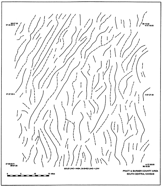
Figure 1 is a map of structural high and low axes taken from a subsurface map with good well control in Pratt and Barber counties, Kansas (Williams, 1968). Figure 2 shows the axes of residual aeromagnetic highs and lows of the same area. These magnetic highs and lows reflect the lithology of the basement rocks because of differences in the magnetite content of the igneous and metamorphic rocks comprising the basement. These rock type changes and the generally sheared boundaries between them control the basement topography. Note the great similarity of the patterns in the two figures. Quantitative analysis resulted in a 74% correlation factor between the structural and basement alignments on the two maps. This demonstrates the pervasive basement topographic control of the structural axes, both highs and lows, in the lower parts of the sedimentary section in Kansas (and certainly elsewhere, as well).
Figure 1--Axes of Simpson structural highs and lows, taken from Williams (1968).
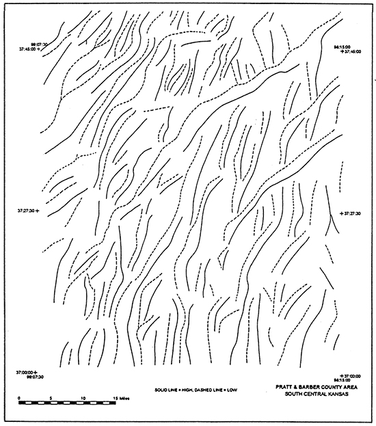
Figure 2--Axes of residual magnetic highs and lows of area of fig. 1, taken from proprietary aeromagnetic basement mapping by Applied Geophysics, Inc., 1982-83.
The above concept opens up the exploration possibilities considerably. Now we must not only think of structural closure appearing over basement highs, we must also consider the possibility of fluvial deposits (Morrow channels, for example) occurring in structural-topographic lows on top of the Mississippian unconformity, or other unconformity surfaces in Kansas.
The second type of basement control, in addition to basement topographic control, is structural control, that is, faulting in the sedimentary section following old, reactivated basement faults. This is an old concept and adheres to the adage that "once a fault, always a fault." However, faults in the basement are not the type of sharp breaks we see in the sedimentary section. They are generally broad shear zones having widths of a half mile to a mile or more. These are the block boundaries of the "basement fault block pattern." Distances between basement shear zones vary considerably but are generally bracketed in the 2-5 mi (3-8 km) range. They occur in sets of parallel to sub-parallel fractures having different strike directions. They are of distinct ages and hence there are frequent terminations and truncations, and they are mappable with detailed residual aeromagnetics because of the rock type changes and magnetic susceptibility changes across them. These shear zones also generally erode low because they are intensely fractured, and this causes them to be visible on Landsat images of exposed basement, such as the Canadian Shield or other shield areas of the world. For emphasis, I summarize the above concepts in table 1.
Table 1--Two basic types of basement control on the overlying sedimentary section.
| 1. Basement Topographic Control. Structure is created in the overlying sedimentary section because of gravitational compaction of the sediments over the irregular basement topography. This results in many stratigraphic phenomena as well. (See, for example, Gay, 1989). |
| 2. Reactivated Basement Faults or Shear Zones. Regional stresses reactivate some of the basement weakness zones, thus localizing structure, as well as causing stratigraphic effects in the overlying sedimentary section. |
Accepting these concepts of basement control, we can now proceed to the next step--the actual use of the concepts in exploration for oil and gas. First of all, in what ways does basement control affect hydrocarbon trapping and reservoir development? An initial attempt at tabulating some of the ways this can occur is given in tables 2 and 3. Nineteen different geological mechanisms are shown. However, this must be considered an abbreviated list. Familiarity with hundreds, or thousands, of oil fields would be necessary for constructing a complete list, if such is possible. For example, in preparation for this paper a new type of reservoir not previously considered was found: oolite shoal development on a sea floor high over a reactivated basement fault (Collier Flats field, Comanche County, as described by Slamal, 1985; see fig. 13).
Table 2--Types of traps and reservoirs resulting from basement topographic control.
Direct
|
Indirect
|
Table 3--Types of traps and reservoirs resulting from basement fault control.
Direct
|
Indirect
|
In order to utilize the above-described concepts of basement control on the structure and stratigraphy of the sedimentary section, it is helpful to understand a certain amount of basement, or Precambrian, geology. As a start, one could examine Landsat or SLAR images of outcropping basement areas worldwide ("shields") to get a feel for what the basement shear zones might look like underneath Kansas. However, it is not necessary to understand the details of Precambrian metamorphic and igneous petrology to grasp and apply basement concepts to exploration. Table 4 is a summary of sufficient information on basement geology to guide an exploration program.
Table 4-Basement fault block pattern--basic concepts.
|
The great complexity of basement structure results from active tectonism over the very long time span of the Precambrian Era, 4 billion years. This is approximately seven times longer than the time from the beginning of the Cambrian to the present. Not only this, but tectonism seems to increase as one goes back in earth time, i.e., plate tectonics is apparently slowing down, in spite of the fact that we are awed by the assemblage and breakup of Gondwana and Laurentia in the last 500 million years. A preliminary analysis of magnetic basement mapping in north-central Oklahoma-south-central Kansas revealed approximately eight major tectonic events that affected the Precambrian crust of the region (Gay, 1986). The great majority of these events, six and perhaps more, took place prior to 1.4 billion years ago. An emerging concept among students of Precambrian geology is that all the continents contain pieces of all the other continents due to the hectic pace of plate tectonics in the early stages of earth's history.
Some probable early Precambrian plate boundaries are visible in the residual magnetic data of the midcontinent region. Figure 3A is a banded contour version of residual magnetic data in south-central Kansas, covering approximately 3° of longitude and 1° of latitude. This figure is a regional map of the same magnetic data that are shown in the individual oil-field examples, figs. 4 through 13. It is made up of alternating bands of black, gray, and white between magnetic contour lines, rather than using the contour lines themselves. This type of presentation could also be called "variable density magnetics" and is extremely useful for seeing regional trends, or "sutures," in magnetic data.
Figure 3A (top)--Banded contours of residual magnetic map of part of south-central Kansas. Note the four obvious basement sutures (tectonic boundaries), as indicated by the arrows. Figure 3B (bottom)--Names are given for the various Precambrian terranes that are separated by the indicated sutures (from Gay, 1986, reproduced by permission of the Basement Tectonics Association). In the present paper, the sutures themselves are given names-A-A', Argonia Suture; B-B', Pratt Suture; C-C', Pretty Prairie Suture; and D-D', Joy Suture. Note the close correlation of the "Yellowstone-Peace Creek Tectonic Zone" (YPCTZ) with the Pratt Suture. It would be surprising if the Argonia Suture has not been similarly reactivated.
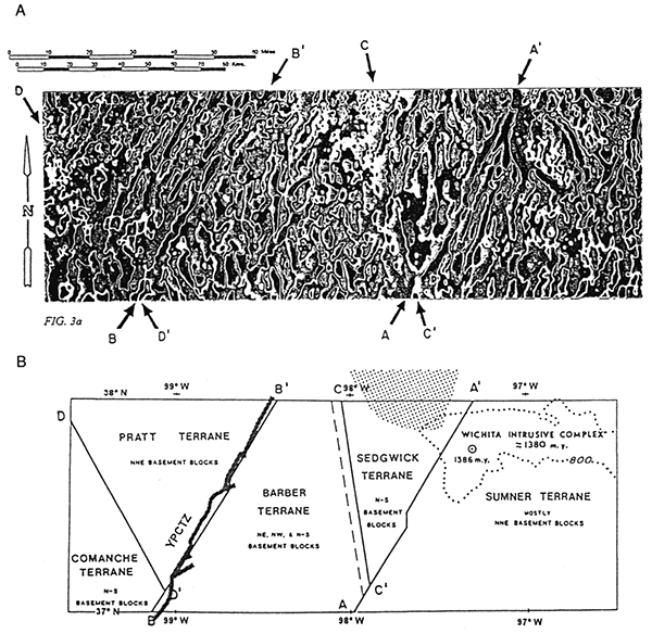
Tectonic boundary A-A' in fig. 3a, herein named the Argonia Suture, separates all northeast-trending basement blocks on the east from all north-trending basement blocks on the west. The area of northeast-trending blocks has previously been named the Sumner Terrane and the area of north-trending blocks the Sedgwick Terrane (fig. 3B) for the counties that fall within them (Gay, 1986). Sixty miles (100 km) to the west lies tectonic boundary B-B', the Pratt Suture, which separates all northwest-trending basement blocks of the Pratt Terrane on the west from the northeast, northwest, and north-south trends of the Barber Terrane on the east. The parallelism of A-A' and B-B' suggest a related origin, and one is reminded of the accreted terranes still active along the west coast of North America from California through Alaska. The ages of the Precambrian tectonic boundaries in fig. 3 must be considerably in excess of an age date of 1,386 Ma obtained within the Wichita intrusive complex shown on the east side of fig. 3, as the intrusive complex seems to be younger than A-A'. Even older are tectonic boundaries, C-C' (Pretty Prairie Suture) and D-D' (Joy Suture) which are truncated by A-A' and B-B' respectively. Certainly all the basement terranes, tectonic boundaries, and individual block boundaries were in place by Cambrian time and would have appeared much as they appear today in fig. 3.
The long strike length and great amount of inferred displacement of the tectonic boundaries in fig. 3 indicate that they are zones of greater than average weakness and as such, should be easily reactivated by later stress systems. This appears to be the case for the Pratt Suture, which is almost exactly coincident with the Pratt anticline or "Yellowstone-Peace Creek Tectonic Zone" (Berendsen and Blair, 1986; Slamal, personal communication, 1992). This is one of many zones in Kansas that are parallel to the Nemaha Ridge and are of latest Mississippian-early Pennsylvanian age. Perhaps such Mississippian-Pennsylvanian disruption also exists along the Argonia Suture (A-A'), but we have not examined subsurface data to investigate that possibility.
As outlined in table 4, basement tectonism juxtaposed rocks of differing magnetic susceptibilities across shear zones long before Cambrian time. It is this fact which allows us to map the shear zones with residual aeromagnetics. The shear zones thus fall on the magnetic gradients between the residual magnetic highs and lows. They are the principal zones of weakness in the basement that were reactivated by later (Paleozoic) tectonic events. Extensive comparison of reliable subsurface and seismic maps over large areas of the midcontinent and the Rocky Mountains at Applied Geophysics, Inc., have shown that fully 65-70% of the faults cutting the sedimentary section in these areas lie on magnetically mapped basement shear zones. Possibly the percentage of correlation would be higher if the mapped fault traces were more exact, but there are also cases where reliably defined faults cut through the interiors of basement blocks rather than following block boundaries. There are few absolutes in geology, but certainly a map of the basement fault block pattern is a good starting point for understanding the structure of an area.
Likewise, a map of the basement fault block pattern is an aid in locating basement topographic features. Basement shear zones (i.e., the edges of basement blocks) generally erode topographically low. That is why they are so evident on Landsat images of outcropping basement. This means that basement topographic highs generally fall within the block interiors, but where? Is the whole basement block a topographic high, is one edge higher, or are there several topographic highs within a single block? It is generally not possible to answer these questions with magnetics. In fact, some basement hills correspond to magnetic lows (see fig. 5). This would be the case where a basement hill is carved on a block that is less magnetic than surrounding blocks. Quartzite is one rock type that falls in the weakly magnetic category, and basement hills of quartzite are not uncommon in Kansas (Waiters, 1953; J. Brewer, personal communication, 1983).
This brings up the problem of the ambiguity of magnetic data for mapping the vertical dimension; for example, attempting to determine whether a basement block is high or low or has a hill on it, or which side of a basement fault is up or down. Since the magnetic pattern is caused by the lithology of the basement rocks, neither of these problems is generally solvable with magnetics, especially in areas of low basement relief and limited fault throw, as in Kansas. In the highly regarded GSA Memoir 47, the first book ever written on aeromagnetic interpretation, it is stated: "Most magnetic anomalies arise from the lithology and not from the topography of the basement rock" (Vacquier et aI., 1951, p. 8). In the third edition of Introduction to Geophysical Prospecting, a similar statement is made: "The magnetic relief observed over sedimentary basin areas is almost always controlled by the lithology of the basement rather than by its topography" (Dobrin, 1976, p. 534). On the other hand, the determination of the edges of magnetic anomalies (i.e., the boundaries of the basement blocks) or the horizontal dimensions, x and y, is not ambiguous.
It is recommended that the vertical dimension (z) be determined from subsurface or seismic data, which is precisely what these techniques measure. Thus, to obtain the best geologic picture of an area in all three dimensions (x, y, and z), one should integrate magnetic basement mapping with seismic and subsurface data. In reality, magnetics, like subsurface studies, must come before seismic, in order to determine the location of the most economic acquisition of seismic data as well as the necessary amount of data to obtain.
How does gravity surveying fit into this picture and when should it be employed? The author feels that in most cases gravity should be used like seismic as a follow-up tool run at a tight station-spacing of 200-500 ft (60-150 m) along specific profile lines, each a few miles long. In many cases, this could indicate whether a basement hill is present or which side of a fault is up. However, gravity is almost never used in this fashion. It is generally run on grids of 1 mi (1.6 km) spacing (sometimes with tighter spacing along roads) to give a regional picture. Here, it competes with aeromagnetics, which does a better and more detailed job of mapping the basement fault pattern. Aeromagnetic readings are spaced from tens of feet apart up to a maximum of 200 ft (60 m) along line, and this high density of data essentially defines the magnetic profile completely. The profile lines can be flown at any line spacing desired but are generally flown at a separation equal to one third to one half the depth to basement.
Many, or most, basement block boundaries are not readily defined by gravity as there is little contrast in the densities of the juxtaposed blocks. Overall, densities of basement rocks vary from about only 2.5 gms/cc to a high of 3.2 gms/cc (in rare cases)--a 28% change. However, magnetic susceptibilities of basement rocks routinely vary from 50 microcgs to about 5,000 microcgs. This is a 100 times change or 10,000%.
The following pages show selected examples of known oil and gas fields in Kansas controlled, or apparently controlled, by basement features. All these examples are relatively clear-cut and straightforward. That is, the magnetic pattern conforms closely to an oil or gas field or some basement structure which apparently controls the subsurface structure or stratigraphy of the field. One could argue that the veracity of the presented cases is not proven and that the correlations may be fortuitous. On the other hand, one could never prove basement control anywhere at any time unless there were many wells to basement on a given trap or structure. Such a situation is unachievable in actual practice due to the limited number of wells to basement, and we must work with available data and the known principles of geology and geophysics to arrive at answers that satisfy the data in a logical manner. For the topographic aspects, it is important to remember scattered cases throughout the Midwest where there were sufficient wells to basement to define individual basement hills and to realize that compaction anticlines ("graviclines") were present in 30 out of 30 cases (Gay, 1989). For the structural aspects, we must keep in mind that about 65% of the well-documented faults in the sedimentary section that occur within the boundaries of aeromagnetic surveys coincide with residual magnetic gradients, that is, on magnetically mapped basement shear zones.
This example shows a structural high that coincides with a residual aeromagnetic high. For this reason it is considered a probable compaction structure ("gravicline") over a basement hill. Similar examples could be presented for Newbury field in Wabaunsee County, Coleman and Lake Creek fields in Montgomery County, Wellington field in Sumner County, and a number of others. Many additional fields correlate with residual aeromagnetic highs, but there is no published information indicating that they are structural fields.
Figure 4--Moore SW field, Pratt County, a probable gravicline, as evidenced by the close correspondence of the Lansing structure contours (black) with the residual aeromagnetic high (gray). Structure is from Hellman (1985).

This example shows a structural high that coincides with a residual aeromagnetic low. Note the near-straight line gradients on west, south, and east on both sets of contours, indicating the existence of a probable underlying basement hill carved in a weakly magnetic basement rock, such as quartzite. Subsequent conversations in Wichita revealed that some exploration groups had previously noted the same phenomenon and used this concept as an exploration tool in Kansas (J. Brewer, personal conversation, 1983). Other similar correlations of structural highs with residual aeromagnetic lows have been noted for Bloom field in Barber County, Rosedale field in Kingman County, and Wiltex field in Harper County.
Figure 5--Willowdale field, Kingman County, a probable gravicline, as evidenced by the close correspondence of the Viola structure contours (black) with the residual aeromagnetic low (gray). Structure is from Cruce (1956).
This is an interesting structure and could have been included with those in the first example (fig. 4) because it falls on a localized magnetic high. However, it is possible to interpret more of the basement geology here since the field falls precisely within a circular area of lower magnetic susceptibility than the area surrounding it. This is especially evident on the 3D stereo pair of the magnetic map. It is thus proposed that the area is underlain by a Precambrian igneous intrusion [4-5 mi (6.4-8 m) in diameter] onto which a basement hill was eroded. A down-to-the-northwest fault cuts all formations older than Pennsylvanian and coincides precisely with a 3- to 5-gamma residual magnetic gradient. This is typical of the fault correlations obtained with basement mapping where reliable geological data exists.
Figure 6--Alameda field, Kingman County, a probable gravicline, as evidenced by the close correspondence of the Viola structure contours (black) with the residual aeromagnetic high (gray). Structure is from King (1965).
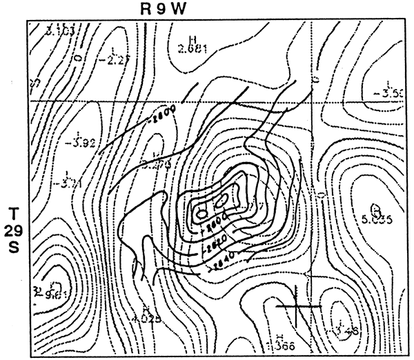
This example is included to illustrate a remarkable fault correlation, but there is reason to suspect that Coats field is a compaction structure over a basement hill. What else would cause a structure in south-central Kansas less than 1 mi (1.6 km) wide to have over 450 ft (135 m) of total vertical displacement on the Arbuckle? (Localized basement "uplift," piston fashion, is not a viable tectonic mechanism.) Realizing that such a basement topographic high probably does exist on the edge of a 3 x 3 mi (4.8 x 4.8 km) wide basement block as mapped by the magnetic high (fig. 7), one might speculate that there is a basement rock type here which erodes to a "knobby" terrain (granite, perhaps?). The four "corners" of this block--NW, NE, SE, and SW--corresponding to the magnetic high thus become interesting places to use subsurface or seismic data to look for other structural highs. What is remarkable in fig. 7 is that the short NNE-trending fault within Coats field and the long seismically mapped fault underlying the Pratt anticline correlate precisely with residual magnetic gradients (i.e., the locations where one draws basement shear zones).
Figure 7---Coats field, Pratt County, a possible gravicline. Other possible graviclines would be the "corners" (noses) of the same magnetic high where Coats field is located. Structure (black) is on top of Arbuckle at a 50-ft (15-m) contour interval and is from Curtis (1956). Note the correlation of the long northeast fault, the deep manifestation of the shallow Pratt anticline, along the "Yellowstone-Peace Creek Tectonic Zone" with the residual magnetic gradients (gray).
If high basement topography causes structural highs in the overlying sedimentary section, then low basement topography must result in overlying structural lows. It is possible then, through the process of erosion, that Mississippian structural lows in western Kansas-eastern Colorado became Pennsylvanian topographic lows. They would thus be favorable sites for the deposition of Morrow channel sands.
Figure 8--Stateline Trend, Wallace and Greeley counties, Kansas, and Cheyenne and Kiowa counties, Colorado, superimposed on residual magnetic contours (gray). This prolific Pennsylvanian Morrow channel avoids residual magnetic highs and follows the magnetic lows and gradient areas, as do many similar channels in southeast Colorado.
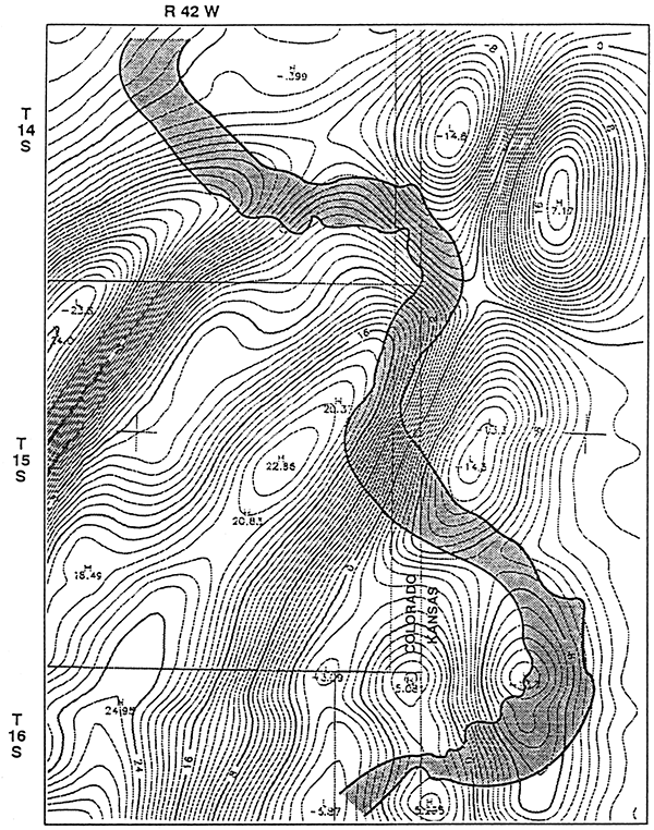
In 1985, one user of residual aeromagnetic data in southeast Colorado found an 85% correlation of Morrow channels with residual aeromagnetic lows. This suggests that there is a rock type in the basement of southeast Colorado that is magnetically weak and erodes topographically low. The Morrow channels there seem to follow magnetic lows and avoid magnetic highs. The subsequently discovered additions of Mt. Pearl and Siaana fields to the Sorrento Trend in Colorado, and the later discovery of the Stateline Trend along the Kansas-Colorado line, substantiated this observation. In fig. 8, the Stateline Trend is seen to bend sharply around a strong northeast-striking residual magnetic high and generally follows the magnetic gradients (i.e., the shear zones, which we expect to erode low) or the magnetic lows themselves. Thus, residual magnetics may be of some value in the search for new channels in the Morrow play, but again, only if integrated or followed up with other geological and geophysical information.
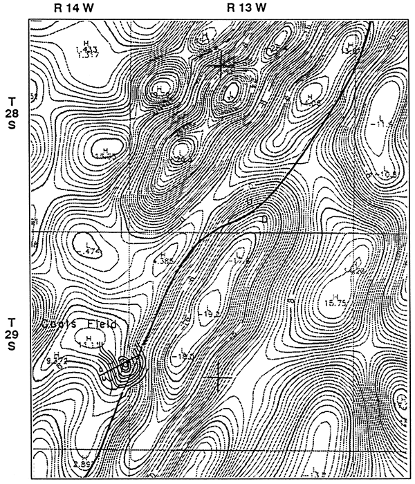
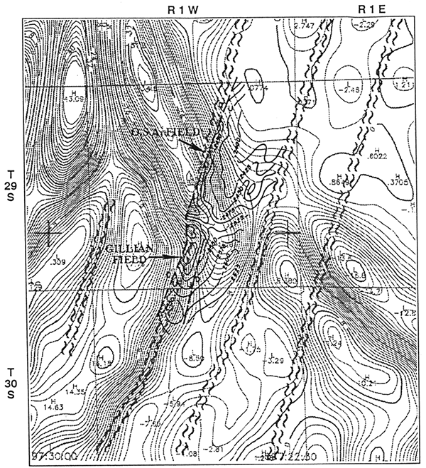
Gillian field has been described as a fault trap on a structurally high horst block (Shawver, 1965a). O.S.A. field is an updip pinchout of the uppermost Simpson sandstone on this same block (Shawver, 1965b). A 1983 interpretation of a residual aeromagnetic survey covering this area precisely defined the west-bounding fault. A series of similar parallel faults, two of which are shown in fig. 9, have been equally well defined by the aeromagnetic data and present additional exploration opportunities. The logical follow-up would be detailed subsurface studies followed by seismic profiling over selected "look-alikes."
Figure 9--Gillian and O.S.A. fields, Sedgwick County. The west fault of Gillian field, which forms the trap, was exactly defined by a 1983 interpretation of the residual aeromagnetic map (gray contours). Structure contours (black) are on top of the Simpson Group, the producing horizon, and are from Sawver (1965a, b).
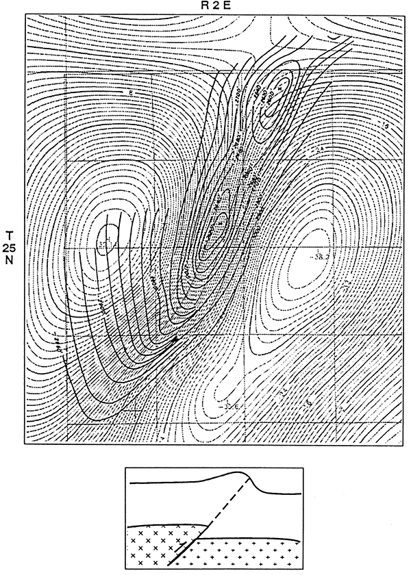
Many truly prolific oil fields have been found along the Nemaha structural system in eastern Kansas and north-central Oklahoma. The Ponca City field in Oklahoma [only 20 mi (32 km) south of the Kansas line] is included in this paper as a remarkable exarnple of such a field. Figure 10 shows the location of the field relative to a strong residual magnetic gradient corresponding to a basement shear zone. Eastward-directed reverse fault movement of the shear zone (as shown in the sketch at the bottom) would explain the asymmetry of the fold. Such fields are common along the Nemaha Ridge, the Beaumont anticline, and other parallel trends in both Kansas and Oklahoma.
Figure 10--Ponca City field, Kay County, Oklahoma. Classic example of an asymmetric fold (black contours) over a basement shear zone defined by the steep gradient in the residual magnetic contours (gray). Reactivation of the shear zone by west-dipping reverse fault movement as in the sketch, is the probable cause of this structure. Mississippi lime structure contours are from Clark and Daniels (1929).
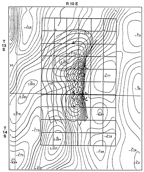
This field [160 mi (256 km) northeast of the Ponca City, Oklahoma, field] is located on the "Alma Trend," which lies 10 mi (16 km) east of, and parallel to, the Nemaha Ridge. Davis Ranch field is a structural look-alike to the Ponca City field and is likewise a large producer falling along a magnetically mapped basement shear zone, although not precisely on it to the south. Auburn and John Creek to the south and Mill Creek to the north are similar fields located over basement faults.
Figure 11--Davis Ranch field, Wabaunsee County. A Kansas analog to Ponca City field (fig. 10), 160 mi (256 km) north of Ponca City in the Alma Trend along the same Nemaha-related fault system. Black contours are top of Viola formation; gray contours are residual magnetics. Structure is from Kansas Oil and Gas Fields, vol. 3, 1960, p. 53.
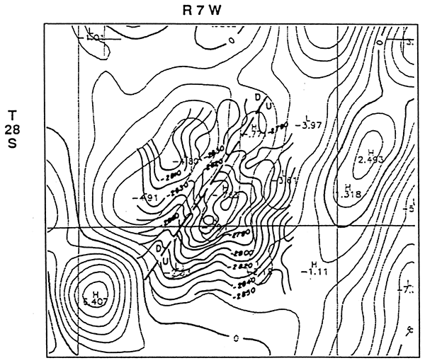
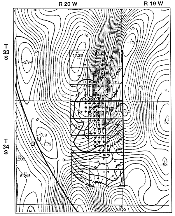
This structural field is similar to the Ponca City field and those of the Alma Trend just mentioned; however, it lies some 75 mi (120 km) west of the Nemaha Ridge along an apparent splay of the Yellowstone-Peace Creek Tectonic Zone. This zone is parallel to the Nemaha Ridge and apparently resulted from the same late-Mississippian compression as the Ponca City and Alma Trend fields. Note the excellent correlation of Cunningham field with the underlying magnetically mapped basement shear zone. Other Kansas fields that seem to fall in the same category are Weathered in Cowley County, North Yellowstone in Comanche County, and Bartholomew in Sedgwick County.
Figure 12--Cunningham field, Pratt and Kingman counties. Close correlation of the underlying basement shear zone with the asymmetric anticline indicates a probable reverse fault here, as in other similar fields in Kansas and Oklahoma. Black contours are on top of the Lansing formation; gray contours are residual magnetics. Structure is from Skelly Oil Company Geology Department, 1956.
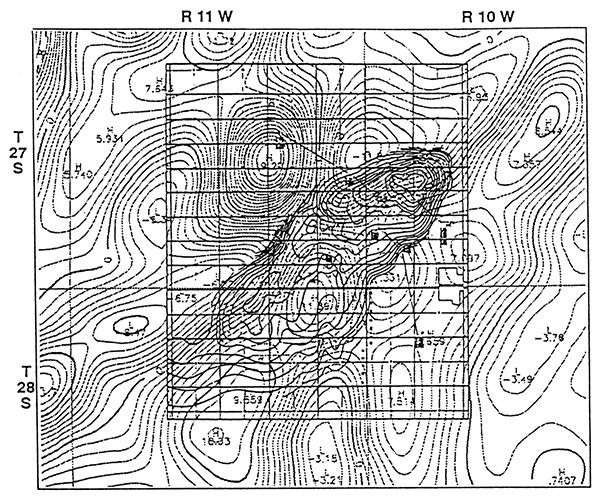
It is fitting to end this suite of field correlations with a stratigraphic example because many times it is stated that structure mapping of the basement is not relevant to certain exploration plays as they are "purely stratigraphic." Some examples of such stratigraphic plays lying along basement faults are the Shannon-Sussex-Ferguson offshore sa~dbars in the Powder River basin in Wyoming, the Muddy fluvial system of the Powder River basin, and the Desert Creek algal mounds of the Paradox basin in Colorado. Siamal (1985) described the Collier Flats field in Comanche County, Kansas, as an oolite shoal that developed on a "structurally high element." The field coincides almost precisely with a magnetically mapped basement shear zone, and Slamal states that this could have been vertically reactivated to produce a sea-floor high that localized the oolite development of Missourian age in the Swope Limestone of the Kansas City Group (Slamal, personal communication, 1992).
Figure 13--Collier Flats field, Comanche County. Production in this field is from an oolite shoal that evidently developed on a fault scarp over an underlying basement fault defined by the gradient in the residual magnetic contours (gray). Structure contours (black) are on top of Pennsylvanian Swope limestone. Structure and wells are from Slamal (1985).
This paper demonstrates two main points:
The first point, that basement control exists, is academic if we cannot map the basement in order to take advantage of basement control. This factor illustrates why point number two is important. There is a means of mapping the basement to some degree, even if that means, residual aeromagnetics, is imperfect. Magnetics cannot locate basement hills with certainty, nor can it be determined which basement shear zones mapped have been offset by faulting and in what direction. Nevertheless, residual aeromagnetics can be used as a starting point, followed in favorable areas with other exploration tools.
In the writer's opinion, the quickest and surest way to use the concept of basement control as an exploration technique is to search for nearby analogs ("look-alikes") to known basement controlled fields. If Collier Flats field, for example, resulted from Pennsylvanian oolite deposition on a fault scarp over a basement fault, is it possible that similar features exist either along strike or on adjacent basement faults? Basement tectonic concepts indicate probable parallel faults two or three miles away on either side, and within this short distance the sedimentary processes may not have changed significantly. If Willowdale field is a gravicline over a basement hill carved in a quartzite block characterized by a residual magnetic low, are there other similar magnetic lows nearby? If Davis Ranch field is an asymmetrical fold over a reverse fault in the basement, surely the stresses caused other such structures along strike (or possibly parallel to it a few miles away).
When Applied Geophysics, Inc., first came to Wichita a decade ago to promote basement mapping with aeromagnetics, several prominent geologists told us: "We're beyond that stage in Kansas." Actually, the reverse appears be true. Many geologists in Kansas and in other parts of the United States have not yet reached "that stage," that is, the stage of understanding that extensive basement control is present in the sedimentary section and that there are ways and means of taking advantage of it. Those geologists who do will certainly discover additional important oil and gas reserves.
The author wishes to acknowledge the continuing encouragement of William A. Miller in the preparation of this paper; the helpful discussions over the years with many Kansas geoscientists, especially R. Walters, A. James, T. Ray, and D. McGuire; and the valuable review and discussions by R. Slamal and D. Baars. The author also is greatly indebted to the staff at Applied Geophysics, Inc. (B. Opfermann, B. Hawley, P. Haslam, R. Andrus, B. Wallin, D. Pap, and F. Benjamin) for their useful assistance and innovative ideas in preparation of this paper.
Berendsen, P., and K. Blair, 1986, Subsurface structural maps over the CNARS with discussion: Kansas Geological Survey, Subsurface Geology Series 8, 20 p., 7 maps [available online]
Blackwelder, E., 1920, The origin of the central Kansas oil domes: American Association of Petroleum Geologists, Bulletin, v. 4, p. 89-94
Clark, S. K., and Daniels, J. I., 1929, Relation between structure and production in the Mervine, Ponca, Blackwell, and south Blackwell oil fields, Kay County, Oklahoma: American Association of Petroleum Geologists, Structure of Typical American Oil Fields, v.I, p. 158- 175
Cloos, H., 1948, The ancient European basement blocks-preliminary note: American Geophysical Union, Transactions, v. 29, no. 1, p. 99-103
Cruce, J. D., 1956, Willowdale Pool: Kansas Geological Society, Kansas Oil and Gas Pools, v. 1, p.95-97
Curtis, G. R., 1956, Coats field: Kansas Geological Society, Kansas Oil and Gas Pools, v. 1, p. 19-24
Dobrin, M. B., 1976, Introduction to geophysical prospecting, third ed.: McGraw-Hill, 630 p.
Gay, S. P., 1985, Gravitational compaction, a neglected mechanism in structural and stratigraphic studies: new evidence from midcontinent, U.S.A.: Applied Geophysics, Inc., Salt Lake City, 109 p.
Gay, S. P., 1986, Relative timing of tectonic events in newly recognized Precambrian terranes in south-central Kansas, U.S.A., as determined by residual aeromagnetic data: Basement Tectonics Proceedings, v. 6, p. 153-167
Gay, S. P., 1989, Gravitational compaction, a neglected mechanism in structural and stratigraphic studies: new evidence from midcontinent, U.S.A.: American Association of Petroleum Geologists, Bulletin, v. 73, p. 641-657
Hellman, T. D., 1985, Moore SW field: Kansas Geological Society, Kansas Oil and Gas Fields, v. 5, p. 175-181
King, C. R., 1965, Alameda field: Kansas Geological Society, Kansas Oil and Gas Fields, v. 4, p. 1-17
Lalicker, C. G., 1949, Principles of petroleum geology: New York, Appleton-Century-Crofts, 377 p.
Mehl, M. G., 1920, The influence of the differential compression of sediments on the attitude of bedded rocks (abs.): Science, New Series, v. 51, p. 520
Moore, R. C., 1920, The relation of the buried granite in Kansas to oil production: American Association of Petroleum Geologists, Bulletin, v. 4, p. 255-261
Shawver, D. D., 1965a, Gillian field: Kansas Geological Society, Kansas Oil and Gas Fields, v. 4, p. 78-87
Shawver, D. D., 1965b, O.S.A. field: Kansas Geological Society, Kansas Oil and Gas Fields, v. 4, p. 175-184
Skelly Oil Co., Geology Department, 1956, Cunningham field: Kansas Geological Society, Kansas Oil and Gas Fields, v. I, p. 25-28
Slamal, R., 1985, Collier Flats field: Kansas Geological Society, Kansas Oil and Gas Fields, v. 5, p.43-52
Taylor, C. H., 1917, The granites of Kansas: Bulletin of the Southwestern Association of Petroleum Geologists, v. 1, p. 111-126
Vacquier, V., Steenland, N. c., Henderson, R. G., and Zietz, I., 1951, Interpretation of aeromagnetic maps: Geological Society of America, Memoir 47, 151 p.
Walters, R. F., 1946, Buried Precambrian hills in northeastem Barton county, central Kansas: American Association of Petroleum Geologists, Bulletin, v. 30, p. 660-710
Walters, R. F., 1953, Oil production from fractured Precambrian basement rocks in central Kansas: American Association of Petroleum Geologists, Bulletin, v. 37, p. 300-313
Williams, C. D., 1968, Pre-Permian geology of the Pratt anticline area in south-central Kansas: M.S. thesis, Wichita State University, 116 p.
Previous--Basement Tectonic Configuration in Kansas || Next--Geophysical Model from Potential-field Data
Kansas Geological Survey
Comments to webadmin@kgs.ku.edu
Web version placed online Aug. 17, 2015. Original publication date 1995.
URL=http://www.kgs.ku.edu/Publications/Bulletins/237/Gay1/index.html