![]()
![]()
![]()
by
Geoffrey C. Bohling and Blake B. Wilson

|
Kansas Geological Survey |
Open-file Report No. 2005-6
Released May 2005
The High Plains aquifer is the primary source of water for the High Plains region of western and south-central Kansas. Some water is also withdrawn from bedrock units, primarily Cretaceous strata, in this region. The Kansas Geological Survey (KGS) and the Kansas Department of Agriculture's Division of Water Resources (DWR) measure water levels in aquifers of the High Plains on an annual basis in a network of over 1300 wells, in order to assist in the management of this vital resource. This report presents the statistical quality control analysis for the High Plains region in Kansas based on data from the 2005 water-level measurement campaign along with geostatistical analyses of the 2005 water-table elevations and water-level changes for the one-year and five-year periods preceding the 2005 measurements. The range of dates for the 2005 measurements was from December 22, 2004, to February 24, 2005, but most of the measurements were made in early- to mid-January 2005. Water levels are measured in the winter so that the water table (or potentiometric surface) will have had a chance to recover from the more transient and localized effects of pumping for irrigation. The measurements are presumed to represent a new "static" water level, with the difference from the previous year's measurements representing the net loss or gain of saturated thickness over the preceding year.
The overall average water-level decline in the High Plains region over the 2004 calendar year was 0.15 feet, considerably less than the average decline for the previous two years (1.18 feet for 2003, 1.9 feet for 2002). This is primarily because 2004 was a relatively wet year after several years of drought, as discussed in Section 9 of this report. However, regions of strong decline still persist in Kearny, Finney, and Gray counties.
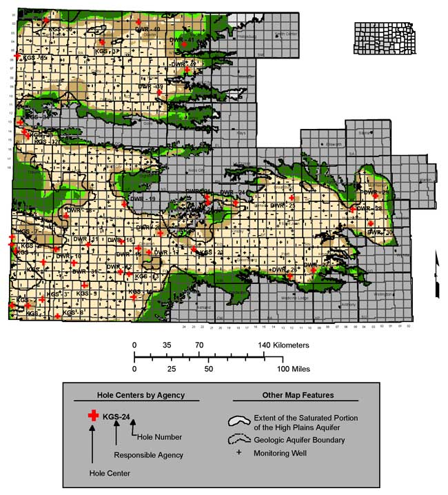
The KGS and DWR traded responsibility for significant portions of the measurement network this year, with the KGS taking over 226 wells in the High Plains aquifer extent previously measured by the DWR and the DWR taking over 166 wells previously measured by the KGS. Figure 1 is a map showing the responsible agency for each well in 2004 and 2005. The KGS is now primarily responsible for measuring wells in the western and southwestern portions of the network, whereas the DWR is responsible for the central and eastern portions. One significant effect of the change is that the DWR is now responsible for measurements in the region that has experienced the highest levels of declines.
Figure 1--2005 county responsibilities and wells measured in 2004 and 2005, by agency.
Throughout this report we refer to water-level declines, with a positive decline meaning an increase in depth to water from the land surface (or decrease in water-table elevation) and a negative decline meaning a decrease in depth to water from the land surface (increase in water-table elevation). This convention makes sense, since falling water levels, and thus positive declines, have historically prevailed throughout the region. However, it is perhaps a little counterintuitive because, in this case, positive numbers indicate a reduction of water in storage while negative numbers indicate an increase.
We would like to thank the external reviewers of this manuscript, Susan Stover of the Kansas Water Office and Tom Huntzinger of the Kansas Department of Agriculture's Division of Water Resources, and the internal (KGS) reviewers, Don Whittemore and Rex Buchanan, for their helpful suggestions for improving this report.
Water-level measurements for the 2005 campaign were extracted from the Water Information Storage and Retrieval Database (WIZARD) database of the Kansas Geological Survey using the SQL statement shown in Listing 1. This query accesses two views, one representing all wells in the measurement network (wizard_network_wells) and the other representing all water-level measurements made in those wells over the years (wizard_network_wells_wl). The query shown in Listing 1 yields 1362 measurements from 1308 distinct wells, with measurement dates ranging from December 22, 2004, to February 24, 2005. Of these, 1267 wells are located within the extent of the saturated High Plains aquifer, 715 measured by DWR personnel and 552 measured by KGS personnel. The wells within the extent of the High Plains aquifer are screened primarily in that aquifer but also include some wells screened only in an alluvial aquifer or in underlying bedrock. The three geologic unit identifiers shown in the Listing 1 (concatenated into the single variable "geol_units") identify up to three different geologic units tapped by each well. The query extracts location data (latitude, longitude, and surface elevation) along with the additional variables used in the statistical quality control analysis. Similar queries were used to extract data from the 2004 and 2000 measurement campaigns for the sake of computing 1-year and 5-year water-level changes.
Listing 1--SQL query for extracting 2005 water-level measurements from WIZARD.
select
    bwilson.wizard_network_wells_wl.*,
    bwilson.wizard_network_wells.land_surface_altitude as surf_elev,
    bwilson.wizard_network_wells.latitude as latitude,
    bwilson.wizard_network_wells.longitude as longitude,
    bwilson.wizard_network_wells.well_access,
    bwilson.wizard_network_wells.downhole_access,
    bwilson.wizard_network_wells.use_of_water_primary,
    bwilson.wizard_network_wells.geological_unit1 ||
    bwilson.wizard_network_wells.geological_unit2 ||
    bwilson.wizard_network_wells.geological_unit3 as geol_units,
    bwilson.wizard_network_wells.local_well_number as kgs_id,
    bwilson.wizard_network_wells.other_identifier as AnnProv
  from
    bwilson.wizard_network_wells_wl, bwilson.wizard_network_wells
  where
    bwilson.wizard_network_wells_wl.usgs_id =
         bwilson.wizard_network_wells.usgs_id and
    bwilson.wizard_network_wells_wl.depth_to_water is not null and
    (bwilson.wizard_network_wells_wl.agency = 'KGS' or
        bwilson.wizard_network_wells_wl.agency = 'DWR' ) and
    bwilson.wizard_network_wells_wl.measurement_date_and_time >=
                '01-Dec-2004' and
    bwilson.wizard_network_wells_wl.measurement_date_and_time <=
                '28-Feb-2005'
  order by
    bwilson.wizard_network_wells_wl.usgs_id,
    bwilson.wizard_network_wells_wl.measurement_date_and_time
For the sake of quality assurance, repeat measurements were made at 53 wells, most within a day of the initial measurement. These measurements indicate a high degree of repeatability in the measured water levels. Figure 2 shows a normal quantile-quantile (QQ) plot of the absolute differences between repeat measurements. A normal QQ plot displays sorted data values plotted against the corresponding quantiles of a standard normal distribution, highlighting deviations from normality and especially the behavior in the tails of the distribution. Normally distributed data with the same mean and standard deviation as the dataset in question would fall along the straight line shown in the plot. Even when we are not particularly concerned about whether the data are normally distributed, normal QQ plots provide a consistent convention for displaying data distributions. Unlike a histogram, the data display in a QQ plot is not obscured by the subjective choice of arbitrary parameters such as bin width and bin origin.
Figure 2--Normal QQ plot of differences between repeat measurements at 53 wells.
The mean absolute difference between first and second measurements is 0.36 feet, 39 of the differences are less than 0.25 feet, and 46 of them are less than 0.5 feet. As indicated in Figure 2, the maximum difference between repeat measurements is 5.8 feet for the well with KGS ID 33S 39W 04DBB 01. The depth to water in this well was measured as 94.51 feet on the morning of January 11, 2005, and as 100.49 feet that afternoon. Both of these measurements are quite out of trend, indicating a water-level rise of about 22 feet in 2004, a behavior that is not reflected in nearby wells. Therefore this well was eliminated from further analysis, leaving 1266 wells.
Summary statistics for the 2005 depth to water (from ground surface) and water-table elevation, along with the declines since 2004 and 2000, are shown in Table 1. In this analysis we used average depth values for those wells with repeat measurements. For the sake of comparison, Table 2 shows the corresponding statistics for the 2004 measurements. It is clear that declines during 2004 were significantly less than those during 2003. Figures 3 and 4 (page 10) show histograms of the one- and five-year water-level declines and Figures 5 and 6 (page 11) are the corresponding normal QQ plots. In keeping with the lower mean decline, the distribution of one-year declines (Figures 3 and 5) is much less skewed towards positive values than in previous years, although there are still more positive declines (716) than negative declines (513).
Table 1--Summary statistics for 2005 water-level measurements and one- and five-year water-level declines.
| 2005 Depth (feet) |
2005 Elevation (feet a.s.l.) |
2004 to 2005 Decline (feet) |
2000 to 2005 Decline (feet) |
|
|---|---|---|---|---|
| Minimum: | -0.18 | 1324.92 | -23.09 | -29.33 |
| 1st Quartile: | 35.03 | 2156.25 | -0.58 | 1.32 |
| Mean: | 113.40 | 2605.12 | 0.15 | 5.47 |
| Median: | 109.52 | 2687.94 | 0.19 | 3.80 |
| 3rd Quartile: | 166.17 | 3038.38 | 0.98 | 7.55 |
| Maximum: | 391.29 | 3837.10 | 18.27 | 42.20 |
| Std. Dev.: | 81.49 | 589.88 | 2.25 | 6.40 |
| Count: | 1266 | 1266 | 1229 | 1167 |
Table 2--Summary statistics for 2004 water-level measurements and previous one- and five-year water-level declines.
| 2004 Depth (feet) |
2004 Elevation (feet a.s.l.) |
2003 to 2004 Decline (feet) |
1999 to 2004 Decline (feet) |
|
|---|---|---|---|---|
| Minimum: | 0.62 | 1325.52 | -16.40 | -19.92 |
| 1st Quartile: | 35.11 | 2150.96 | 0.22 | 1.64 |
| Mean: | 112.66 | 2602.20 | 1.18 | 5.58 |
| Median: | 108.98 | 2680.61 | 0.88 | 3.87 |
| 3rd Quartile: | 165.89 | 3038.30 | 1.94 | 7.38 |
| Maximum: | 391.92 | 3837.34 | 20.74 | 51.08 |
| Std. Dev.: | 80.64 | 590.87 | 2.49 | 6.51 |
| Count: | 1253 | 1253 | 1216 | 1158 |
Figure 3--Histogram of water-level declines between 2004 and 2005 campaigns.
Figure 4--Histogram of water-level declines between 2000 and 2005 campaigns.
Figure 5--Normal QQ plot for one-year water-level declines.
Figure 6--Normal QQ plot for five-year water-level declines.
The wells with the most extreme one-year declines are indicated on Figure 5. The three wells flagged are
| KGS ID | USGS ID | 2004 to 2005 decline (feet) |
|---|---|---|
| 23S 35W 24BBB 02 | 380245101071102 | 18.3 |
| 30S 34W 05BBB 01 | 372825101041201 | 16.1 |
| 29S 35W 24BAA 01 | 373104101060001 | -23.1 |
The first two wells, with the most extreme declines, changed from KGS to DWR measurement responsibility in 2005 but are also in regions of significant decline, so it is difficult to determine whether these extreme values are real or artifacts of the change in responsibility. A network well one mile to the south of well 23S 35W 24BBB 02 showed a decline of 6 feet this year. Another well one mile to the north showed no significant change this year but dropped 18 feet the previous year (2003-2004). Well 29S 35W 24BAA 01, with the largest water-level increase (negative decline), is a DWR well with some history of being difficult to measure, but the WIZARD entry for it does not contain any notes about difficulties this year. Oddly, this well is only 3.3 miles from 30S 34W 05BBB 01, the well showing the second largest decline.
The six wells with the most extreme five-year changes, indicated on Figure 6, are:
| KSG ID | USGS ID | 2000 to 2005 decline (ft) |
|---|---|---|
| 26S 41W 32DDB 01 | 374421101490901 | 42.2 |
| 24S 33W 18BDB 02 | 375812100591302 | 38.1 |
| 24S 33W 19DBB 02 | 375706100585702 | 35.6 |
| 27S 32W 06CBB 01 | 374343100520801 | 35.3 |
| 15S 42W 32BDA 01 | 384238102004501 | -15.8 |
| 18S 38W 23BAB 01 | 382851101291601 | -29.3 |
There is a two-year gap in the record (2002 and 2003) for well 26S 41W 32DDB 01 and it is labeled as tapping undifferentiated Cretaceous and Jurassic formations. Wells 24S 33W 18BDB 02 (measured twice in 2005) and 24S 33W 19DBB 02 both tap the Cretaceous Dakota aquifer and have a history of highly oscillatory water levels. Well 27S 32W 06CBB 01 shows a very steady decline, but just changed hands from KGS to DWR. Responsibility for wells 15S 42W 32BDA 01 and 18S 38W 23BAB 01, the highest five-year water-level increases, also just switched from DWR to KGS. This almost gives the impression that DWR measurements tend to be deeper than KGS measurements, but any systematic differences in measurement processes between the two agencies would be obscured by the fact that DWR took over responsibility for the areas of most extreme decline, as discussed above.
The statistical quality control is based on analysis of variance of water-level declines between the 2004 and 2005 measurement campaigns versus a number of categorical variables describing various aspects of the measurement process and characteristics of the well. These variables include the initials of the measurer, the ease or difficulty of accessing the well, whether a weighted tape was used in the measurement, the primary use of the well, whether oil was present on the water, the chalk cut quality for the measurement, and a code indicating which aquifer(s) provide the primary source of water for the well. Ideally, none of these factors should have a systematic effect on the measured declines except possibly the formations tapped by the well.
The analysis is based on one-year declines, rather than the measured depth to water, in order to factor out the predominant influence of the spatial location on the water-level measurement. However, the observed declines also display spatial correlation and some of the variation between factors analyzed here could be confounded with that spatial correlation. Therefore, an analysis of variance based on residuals from the kriged estimate of one-year declines is presented in Section 8 of this report.
This analysis uses differences between 2005 and 2004 depths to water for wells located within the High Plains aquifer extent measured by KGS personnel in 2005, excluding well 33S 39W 04DBB 01, the one that exhibited the 5.8-foot difference between repeat measurements, resulting in a total of 534 wells. For the 49 wells with repeat measurements in 2005, we used the first measured depth, rather than the average depth, in order to avoid ambiguity in the assignment of measurer. However, for wells with repeat measurements in 2004 we used the average measured depth in the computation of the one-year declines.
The values taken on by the analysis variables, together with counts of the number of occurrences of each value, are as follows:
| Measurer: | BAW (73), BBW (78), BE (83), DRL (86), JMA (82), JMH (83) JTD (33), RDM (16) |
| Downhole Access: | Easy (290), Hard (244) |
| Weighted Tape: | No Weight (59), Weight (475) |
| Well Use: | H: household water supply (6) I: irrigation (430) N: industrial (2) S: stock water supply (19) U: unused observation (76) Z: animal waste disposal (1) |
| Oil on Water: | No Oil (466), Oil Present (68) |
| Chalk Cut Quality: | Excellent (424), Good (92), Fair (18) |
| Aquifer Code (Geol.Units): |
KD: Cretaceous Dakota (16) KJ: undifferentiated Cretaceous/Jurassic (8) QA: Quaternary alluvium (33) QAQU: Quaternary alluvium + undifferentiated Quaternary aquifers (4) QATO: Quaternary Alluvium + Tertiary Ogallala (6) QU: Quaternary undifferentiated (4) QUTO: Quaternary undifferentiated + Tertiary Ogallala (122) QUTOJM: Quaternary undiff. + Tertiary Ogallala + Jurassic Morrison (1) QUTOKD: Quaternary undifferentiated + Ogallala + Dakota (13) QUTOKJ: Quaternary undifferentiated + Ogallala + Cretaceous/Jurassic (12) TO: Tertiary Ogallala (311) TOKD: Tertiary Ogallala + Cretaceous Dakota (311) |
The results for the analysis of variance are shown in Table 3.
Table 3--Analysis of variance using twelve aquifer codes (Geol. Units)
| Source | Df | Sum of Sq | Mean Sq | F Value | Pr > F |
|---|---|---|---|---|---|
| Measurer | 7 | 26.29 | 3.754 | 0.9328 | 0.48051 |
| Downhole.Access | 1 | 2.67 | 2.670 | 0.6634 | 0.41574 |
| Weighted.Tape | 1 | 0.15 | 0.146 | 0.0364 | 0.84884 |
| Well.Use | 5 | 33.00 | 6.600 | 1.6398 | 0.14777 |
| Oil.On.Water | 1 | 0.45 | 0.449 | 0.1116 | 0.73850 |
| Chalk.Cut.Quality | 2 | 4.33 | 2.165 | 0.5380 | 0.58427 |
| Geol.Units | 11 | 92.45 | 8.405 | 2.0883 | 0.01971 |
| Residuals | 505 | 2032.410 | 4.025 | ||
| Residual standard error: 2.01 feet | |||||
None of the factors appears to contribute significant variation except for the geological units tapped by the well, and this is only marginally significant. The F value for this factor is 2.09 and the probability of obtaining a greater F value by chance is 1.97%, meaning the variation would be deemed significant at the 5% level but not at the 1% level.
We also ran an analysis of variance using the five-part aquifer classification employed in the 1997 through 2003 analyses. The five-part grouping (Aq.Group5) is obtained from the twelve-part Geol.Units as follows:
| Aq.Group5 | Geol.Units | data count |
|---|---|---|
| QA (Quaternary) | QA, QAQU, QU | 41 |
| QT (Quaternary + Tertiary) | QATO, QUTO | 128 |
| TO (Tertiary Ogallala) | TO | 311 |
| QK (Quaternary-Jurassic) | QUTOKD, QUTOKJ, TOKD, QUTOJM | 30 |
| KK (Cretaceous) | KD, KJ | 24 |
The data counts in the different categories are quite different from those for last year's measurements (Bohling and Wilson, 2004) due to the change in responsibility for different parts of the network between the KGS and DWR. This change results primarily in an increase in the number of KGS wells designated TO and a decrease in the number designated QUTO. The analysis of variance using the five-part aquifer grouping is shown in Table 4.
Table 4--Analysis of variance using five-part aquifer grouping (Aq.Group5)
| Source | Df | Sum of Sq | Mean Sq | F Value | Pr > F |
|---|---|---|---|---|---|
| Measurer | 7 | 26.28 | 3.754 | 0.9400 | 0.47497 |
| Downhole.Access | 1 | 2.67 | 2.670 | 0.6685 | 0.41394 |
| Weighted.Tape | 1 | 0.15 | 0.146 | 0.0366 | 0.84827 |
| Well.Use | 5 | 33.00 | 6.600 | 1.6525 | 0.14449 |
| Oil.On.Water | 1 | 0.45 | 0.449 | 0.1124 | 0.73753 |
| Chalk.Cut.Quality | 2 | 4.33 | 2.165 | 0.5421 | 0.58184 |
| Aq.Group5 | 4 | 80.07 | 20.018 | 5.0124 | 0.00057 |
| Residuals | 512 | 2044.79 | 3.994 | ||
| Residual standard error: 2.00 feet | |||||
As was also true last year (Bohling and Wilson, 2004), grouping the twelve aquifer codes into the five-part classification results in greater significance for that factor, but does not significantly alter the results for any other factor. We also performed an analysis of variance using a six-part grouping in which the eight wells with geological unit designations QU (Quaternary undifferentiated) and QAQU (alluvium plus undifferentiated) were broken out into a separate group from the 33 wells tapping strictly Quaternary alluvium (QA) on the presumption that the strictly alluvial wells might exhibit different behavior from the others. However, the results for that analysis were not significantly different from that for the five-part grouping. In fact, the declines observed in the eight QU and QAQU wells fall solidly in the middle of the distribution for the QA wells, so this result is not surprising.
The global mean decline for the 534 KGS measurements is 0.065 feet and the expected values (least-squares means predicted by the ANOVA model) for each level of each factor are listed below. The expected values for all factors are listed for the sake of completeness. However, it should be kept in mind that the only variation deemed significant by the analysis is the variation between aquifer groups.
| Measurer | ||||||||
| Level | BAW | BBW | BE | DRL | JMA | JMH | JTD | RDM |
|---|---|---|---|---|---|---|---|---|
| Mean | -0.059 | -0.004 | -0.279 | 0.407 | 0.152 | -0.019 | 0.360 | 0.295 |
| Count | 73 | 78 | 83 | 86 | 82 | 83 | 33 | 16 |
| Downhole.Access | ||
| Level | Easy | Hard |
|---|---|---|
| Mean | 0.13 | -0.01 |
| Count | 290 | 244 |
| Weighted.Tape | ||
| Level | No Weight | Weighted |
|---|---|---|
| Mean | 0.11 | 0.06 |
| Count | 59 | 475 |
| Well.Use | ||||||
| Level | H | I | N | S | U | Z |
|---|---|---|---|---|---|---|
| Mean | -0.68 | 0.06 | 0.19 | 0.28 | 0.19 | -5.14 |
| Count | 6 | 430 | 2 | 19 | 76 | 1 |
| Oil.On.Water | ||
| Level | No Oil | Oil Present |
|---|---|---|
| Mean | 0.08 | -0.01 |
| Count | 466 | 68 |
| Chalk.Cut.Quality | |||
| Level | Excellent | Good | Fair |
|---|---|---|---|
| Mean | 0.08 | 0.10 | -0.41 |
| Count | 424 | 92 | 18 |
| Aq.Group5 | |||||
| Level | QA | QT | TO | QK | KK |
|---|---|---|---|---|---|
| Mean | -0.17 | -0.41 | 0.36 | -0.09 | -0.63 |
| Count | 41 | 128 | 311 | 30 | 24 |
Figure 7 shows the water-level declines plotted against aquifer group, the only factor deemed significant by the analysis. Figure 8 is a normal QQ plot of the residuals from the ANOVA model; large residuals indicate decline values that are most out of line with expectations based on the analysis variables (meaning primarily the aquifer group code, in this case). The same six wells are flagged on both plots and listed below.
Figure 7--2004 to 2005 water-level declines by aquifer group.
Figure 8--Normal QQ plot of residuals from ANOVA using 5-part aquifer grouping.
| KGS ID | USGS ID | Decline (feet) |
Residual (feet) |
|---|---|---|---|
| 20S 38W 17CBD 01 | 381840101324401 | 7.07 | 6.84 |
| 34S 36W 10CAC 01 | 370604101132901 | 6.93 | 6.66 |
| 30S 39W 23BBB 01 | 372550101333801 | -11.83 | -11.24 |
| 18S 38W 23BAB 01 | 382851101291601 | -11.99 | -11.57 |
| 34S 35W 10BCC 01 | 370620101071301 | -12.11 | -11.56 |
| 27S 23W 28AAA 01 | 374035099500101 | -12.40 | -12.08 |
This list does not include the three wells with the most extreme one-year declines shown in Figure 5 because those are DWR wells and the present analysis involves only KGS wells. The last well in the list, 27S 23W 28AAA 01, has a history of being difficult to measure and has shown erratic water levels over the past two decades. However, it was measured twice this year, yielding the same result (a water depth of 60.38 feet) both times. Well 34S 35W 10BCC 01 has only been measured since 2003 and has shown significant increases in water level each year. It is surrounded by wells showing water-level rises of three feet or more. Well 18S 38W 23BAB 01 has shown oscillatory behavior over the years. Well 34S 36W 10CAC 01 was measured twice this year, with a difference of only 0.02 feet between the measurements and well 30S 39W 23BBB 01 was measured three times, all with fair chalk cut values and yielding depths of 156.92, 156.17, and 155.85 feet.
For the geostatistical analysis of 2005 water-table elevations, we employed the measurements from both the DWR and KGS at 1266 wells located within the High Plains aquifer extent, using the average values for the 52 wells with repeat measurements. Again, we excluded well 33S 39W 04DBB 01, which shows a difference of almost 6 feet between repeat measurements on the same day and is out-of-trend relative to nearby wells.
As in previous years, we attempted to account for the strong trend in water-table elevation by identifying a trend-free direction, roughly parallel to contours of constant elevation (Olea and Davis, 2003; Bohling and Wilson, 2004). The variogram computed in the trend-free direction is assumed to represent the random, spatially autocorrelated component of the overall variation and the kriging analysis combines this random field model with a first-order local trend model to estimate the water-table elevation at all points on a regular grid. Figure 9 shows directional variograms for a series of azimuths, N 0° E to N 27° E in 1° increments. As for the past two years, the variogram for the direction N 12° E seems to exhibit fairly trend-free behavior, leveling off to a sill of about 12000 sq ft at a separation distance (lag) of about 63 km. The sill of a trend-free variogram represents the overall level of variability of the "random" component of a measured quantity. The increase in variogram values from the nugget, at small lags, to the sill, at a lag value referred to as the range, corresponds to a decrease in correlation between pairs of measurements with increasing separation distance. Measurements separated by distances greater than the range are essentially uncorrelated.
Figure 9--Directional variograms for 2005 water table elevation, computed for N 0° E to N 27° E in 1° increments (azimuths above each plot).
Figure 10 shows the empirical variogram for N 12° E, with two Gaussian models, the one fitted to the 2005 empirical variogram represented by the data points and, for comparison, the model fitted to the empirical variogram for the 2004 water-table elevation data (Bohling and Wilson, 2004). We fitted the variogram models using the weighted least-squares regression procedure described by Olea (1996). The two models produce almost identical results for the shorter lags, indicating that the observed shorter-scale variation was quite similar for 2004 and 2005, but the 2005 model shows a slightly higher sill. The most significant difference for the subsequent analysis, though, is that the estimated nugget value for the 2005 variogram is slightly higher than that for the 2004 model. The square root of the nugget value (13 feet for 2005, 12 feet for 2004) essentially sets the lower limit of the kriging error (standard deviation) for the map used to determine the location of "holes" in the well network. Thus, either of these nugget values precludes the use of the 10-foot standard deviation threshold used in previous years. Therefore, as in last year's analysis (Bohling and Wilson, 2004), we will use a revised threshold standard deviation value to identify network holes.
Figure 10--Empirical variogram in direction N 12° E for 2005 water table elevations, together with Gaussian model fitted to this variogram and Gaussian model fitted to 2004 water-table elevation data (Bohling and Wilson, 2004).
Figure 11 shows the results of the kriging crossvalidation analysis for the 2005 water levels. For this analysis, each well is removed in turn from the dataset, the water level at that location is estimated from surrounding measurements, and the estimated and actual measured values are compared. As would be expected for a smooth surface that has been densely sampled, the correlation between estimated and actual water table elevations is quite high (0.9993) and the root-mean squared (rms) error is quite low (22 feet) relative to the range of elevation values. However, this plot is a little deceptive in that the larger errors (up to 245 feet, Figure 12) would certainly not be considered small when considered as an error in a local estimate of water-table elevation.
Figure 11--Kriging crossvalidation results for 2005 water-table elevations.
Figure 12 is a normal QQ plot for the kriging crossvalidation errors. A positive error means that the estimated water-table elevation, interpolated from measurements at surrounding wells, is higher than the measured elevation at the well, while a negative error means the opposite. Thus, the measured water-table elevation in a well with a large positive error is significantly lower than would be expected based on the elevations observed in nearby wells. This could indicate a significant error in the measurement at the well or a real effect, such as the presence of a significant vertical gradient between the units tapped by the well in question and those tapped by its neighboring wells.
Figure 12--Normal QQ plot of kriging crossvalidation errors for 2005 water-table elevations.
The wells with kriging errors greater than 100 feet in magnitude, flagged in Figure 12, are:
| KGS ID | USGS ID | Kriging residual (feet) |
Geol.Units |
|---|---|---|---|
| 23S 26W 07CCC 01 | 380335100132701 | 245 | KD |
| 23S 40W 29DDB 01 | 380105101433601 | 152 | KD |
| 27S 40W 08CCC 01 | 374240101424201 | 117 | QUTO |
| 25S 25W 32CDD 01 | 374936100052801 | 113 | KD |
| 26S 23W 10DAD 01 | 374725099485601 | 103 | KD |
| 17S 42W 28DAB 01 | 383247101573601 | -104 | TO |
| 21S 39W 07CBA 01 | 381422101385501 | -115 | TO |
| 28S 37W 33DDC 01 | 373346101215801 | -126 | QUTO |
Four of the five largest positive errors are associated with wells tapping the Cretaceous Dakota aquifer. The well with the largest error, 23S 26W 07CCC 01, is a Dakota aquifer well (near the edge of the High Plains aquifer extent) showing a water-table elevation of 2302 feet above sea level. The three nearest neighboring wells tap the Ogallala aquifer (primarily--one is also listed as tapping Quaternary deposits) and have water-table elevations of 2549, 2507, and 2578 feet above sea level. These three measurements contribute most to the elevation estimate at well 23S 26W 07CCC 01 and the estimated value of 2547 feet above sea level is very close to their average (2545), leading to a kriging error of 245 feet. Similar circumstances apply for wells 23S 40W 29DDB 01 and 25S 25W 32CDD 01. Thus the kriging errors for these three wells are almost certainly due to a distinct difference in potentiometric level between the Dakota and Ogallala aquifers in the vicinities of these wells.
Conversely, well 28S 37W 33DDC 01, which shows the largest negative residual, has a measured water table elevation of 2927 feet above sea level but the five nearest wells all have water table elevations around 2800 feet, leading to an estimated water table elevation of 2801 feet above sea level. Of these five nearby wells, the three nearest are listed as QUTO wells, like 28S 37W 33DDC 01, but the next two are listed as TOKJ (Tertiary Ogallala plus undifferentiated Cretaceous/Jurassic). Again, it seems quite possible that well 28S 37W 33DDC 01 could be sampling a distinctly different potentiometric surface than that sampled by the neighboring wells. However, this is also a new provisional well.
Well 17S 42W 28DAB 01 was not pumped in 2004 due to hail damage to the crops. The depth to water here is also very shallow (25 to 30 feet), which lends itself to greater recharge potential. Well 21S 39W 07CBA01 was measured twice on the same day at 184.69 and 184.72 feet water depth.
An analysis of variance for the kriging errors at wells measured by KGS personnel versus the same set of exogenous variables used in the quality control analysis reveals a highly significant variation across aquifer group (using the five-part group), a significant effect due to well use, and a marginally significant influence of chalk cut quality. The least-squares mean residuals predicted by the ANOVA model for these three factors are:
| Aq.Group5 | QA | QT | TO | QK | KK |
|---|---|---|---|---|---|
| Mean | 9.04 ft | -4.36 ft | -2.30 ft | 7.44 ft | 30.61 ft |
| Count | 40 | 128 | 311 | 30 | 24 |
| Well.Use | H | I | N | S | U | Z |
|---|---|---|---|---|---|---|
| Mean | -24.89 ft | 1.43 ft | 3.85 ft | -2.43 ft | -5.75 ft | 47.39 ft |
| Count | 6 | 430 | 2 | 19 | 75 | 1 |
| Chalk.Cut.Quality | Excellent | Good | Fair |
|---|---|---|---|
| Mean | 0.03 ft | -2.16 ft | 12.90 ft |
| Count | 423 | 92 | 18 |
Again, a positive kriging residual indicates that the estimated water-table elevation at a well, interpolated from elevations at surrounding wells, is higher than the observed water table elevation at that well and thus that the observed depth to water in that well is greater than might be anticipated based on surrounding wells, and vice versa for a negative kriging residual. The highly unbalanced nature of the experimental design in this case (large variations in number of measurements for different factor levels) makes it difficult to assess the true significance of the effects, especially for well use, where the residual value for the one waste disposal (Z) well is vastly different than the means for the other factor levels.
Figure 13 shows the crossvalidation errors split out by aquifer group for all wells measured (both KGS and DWR). The extreme residual values flagged are the same as those in Figure 12.
Figure 13--Kriging crossvalidation errors for 2005 water-table elevations versus aquifer group at wells measured by KGS personnel.
Figure 14 is the map of kriged 2005 water-table elevations and Figure 15 is the corresponding error map expressed in terms of the standard deviation of the kriging estimate. Due primarily to the high nugget value of the fitted variogram model for the 2005 data (Figure 10), the kriging standard deviation is at least 13 feet almost everywhere in the network, meaning that the 10-foot standard deviation threshold used to identify network holes in previous years cannot be applied to this year's map. As discussed in Bohling and Wilson (2004), the fundamental information conveyed by the standard deviation map has to do with the spatial distribution of the measurement points; the standard deviation map can be thought of roughly as a map of the distance from an estimation location to the nearest measurement point, scaled according to the variogram model. Although the water-level estimates themselves are fairly insensitive to changes in the variogram, the standard deviation map can change drastically with seemingly small changes in the variogram model, particularly at shorter lags.
Figure 14--Kriged water table elevation for the4 2005 measurement campaign.
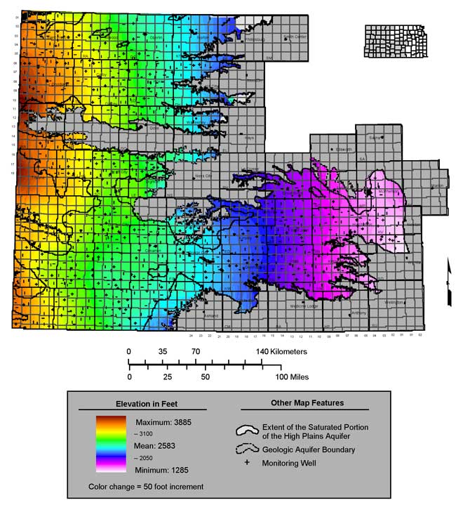
Figure 15--Kriging standard deviation for 2005 weater table elevations.
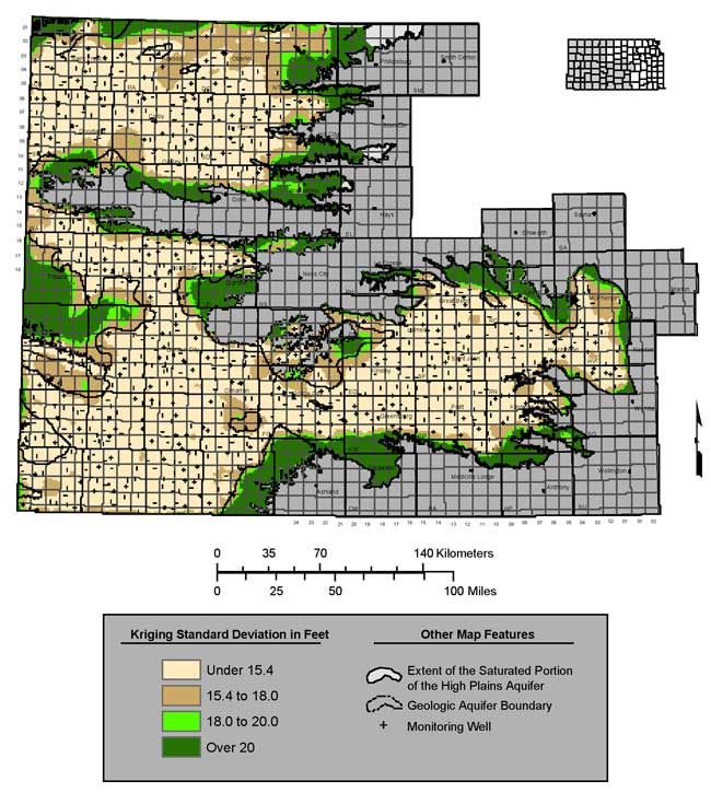
As a point of reference, we applied the model developed for the 2003 water-level data (Olea and Davis, 2003) to the current distribution of well locations. The 2003 model, showing a lower overall variability and particularly a lower nugget effect (67 sq ft), produces a standard deviation below 10 feet throughout most of the network. The 15.4-foot standard deviation contour highlighted in Figure 15 corresponds to the 10-foot contour that would result if we applied the 2003 variogram model to the current distribution of well locations, rather than the 2005 variogram model. We will use this 15.4-foot contour in the identification of network holes discussed in Section 9.
Figure 16 shows the omnidirectional semivariogram for the water-level changes over the five-year period from 2000 to 2005, with an exponential semivariogram model fitted using weighted nonlinear least squares (Olea, 1996). The nugget for this model, 8.8 sq ft, is lower than that for the declines between 1999 and 2004, 17.3 sq ft, meaning that the declines over the five-year period prior to 2005 seem to exhibit somewhat less very short-scale variability than those over the five-year period prior to 2004. However last year's best-fit variogram model for 5-year declines was spherical rather than exponential (Bohling and Wilson, 2004). This exponential model rises more quickly than the spherical model, so that this year's model exhibits somewhat higher variability--or lower correlation--at lags of 20 to 60 km.
Figure 16--Omnidirectional semivariogram for changes in water level over the five-year period from 2000 to 2005.
Figure 17 shows the results of the kriging crossvalidation analysis for the water-level declines between 2000 and 2005. Compared to the water-table elevations, the water-level declines exhibit considerably more short-scale variation relative to their overall level of variation. That is, the map of declines is much less smooth than the map of water-table elevations. Therefore, there is considerably more scatter in the crossvalidation results for the declines than for the water-table elevations (Figure 11).
Figure 17--Kriging crossvalidation results for 5-year water-level changes.
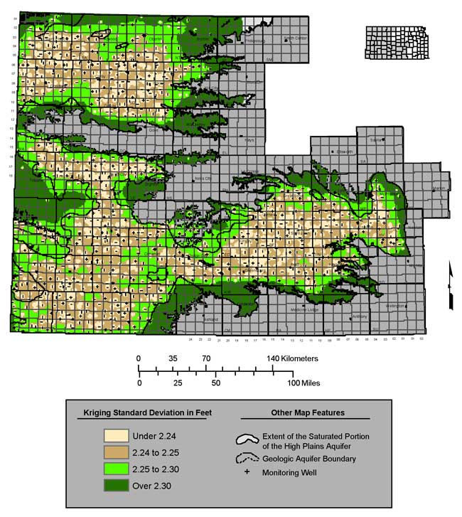
The kriged map of water-level declines between 2000 and 2005 is shown in Figure 18 and the corresponding kriging standard deviation map is shown in Figure 19. Overall, the map of 2000 to 2005 declines is very similar to the map of 1999 to 2004 declines (Bohling and Wilson, 2004), as one would expect. The five-year averaging window means that this map should change very gradually on a year-to-year basis.
Figure 18--Kriged water level declines fo the five-year period from 2000 to 2005.
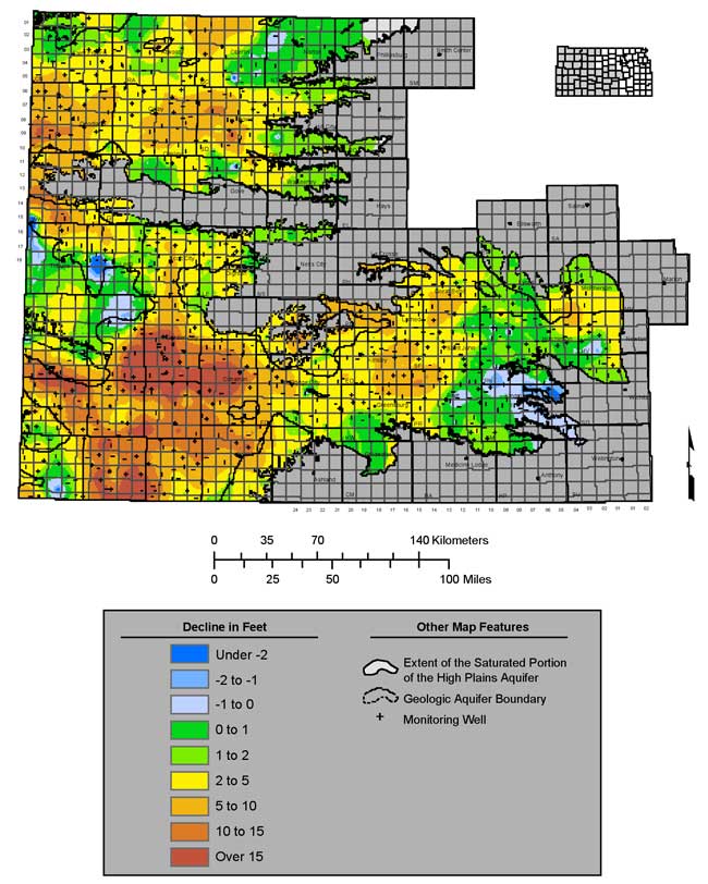
Figure 19--Kriging standard deviation for 2000 to 2005 water level declines.
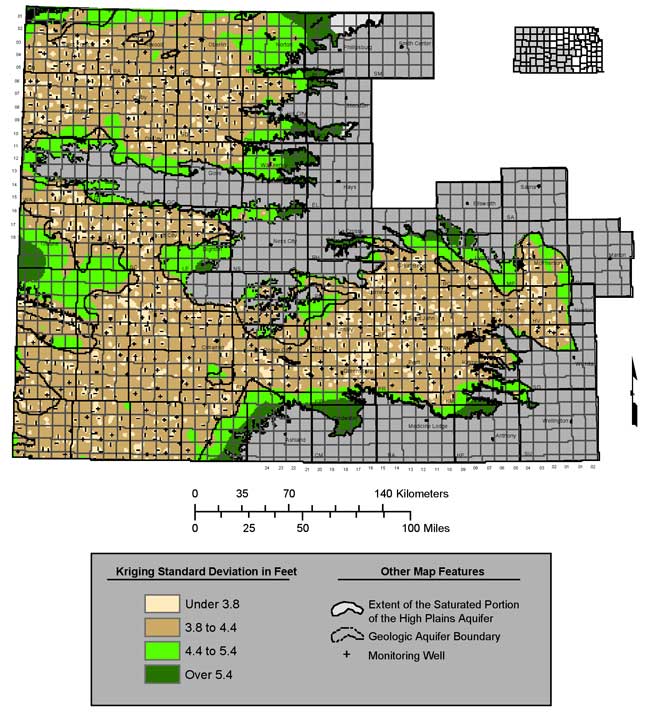
Figure 20 shows the omnidirectional semivariogram for the water-level changes from 2004 to 2005, along with the best-fit semivariogram model, which is spherical in this case. The nugget for this model, 4.49 sq ft, constitutes 77% of the total sill, 5.80 sq ft, meaning that the one-year declines show an extremely high level of short-scale variation. As shown in Figure 21, this results in very low correlation (0.31) between the estimated and actual one-year declines at the wells in the kriging crossvalidation analysis. In this case the smoothing effect of kriging becomes very apparent, with the estimated values showing a considerably narrower range of variation than the actual values.
Figure 20--Omnidirectional semivariogram for changes in water level between 2004 and 2005 measurement campaigns.
Figure 21--Kriging crossvalidation results for changes in water level between 2004 and 2005.
An analysis of variance of the kriging crossvalidation errors for the one-year declines at KGS-measured wells versus the same exogenous variables used in Section 5 shows no significant dependence on any of these factors. Analyzing the kriging errors should help to factor out the spatial dependence that would possibly be confounded with some of the factors in the ANOVA of the decline values themselves. As with the 2004 analysis, the lack of systematic dependence of the kriging errors on the exogenous variables is persuasive evidence that the measurement program is providing high-quality data.
Figure 22 is the kriged map of water-level declines from 2004 to 2005 and Figure 23 is the corresponding standard deviation map. On a regional level, the higher decline areas from 2004 to 2005 in Sherman, Thomas, Sheridan, Wallace, Kearny, Finney, and Ford counties roughly mirror areas with relatively higher reported ground-water use regions (Wilson et al., 2002) and have historically shown greater levels of decline over time. Of particular interest, areas of eastern Stevens and western Seward counties showed notable rises from 2004 to 2005 in the water table. This is a continuation of a trend first identified from 2003 to 2004 (Bohling and Wilson, 2004). The kriged map of water-level declines also shows widespread rises in the water table in areas of the Great Bend Prairie and Equus Beds aquifers of south-central Kansas.
Figure 22--Kriged water level declines from 2004 to 2005.
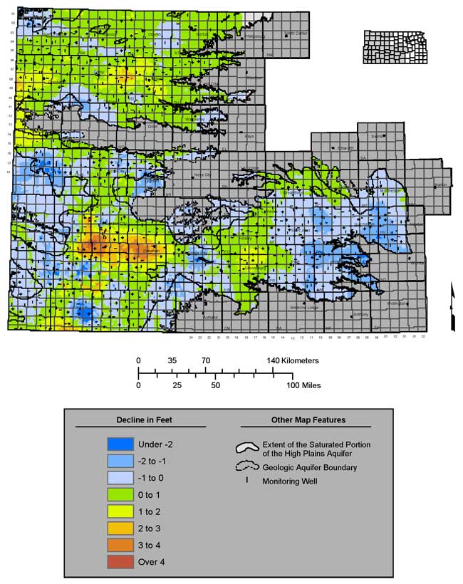
Figure 23--Kriging standard deviation for 2004 to 2005 water level declines.
The regional average of the water-level decline for 2004, 0.15 feet, is the lowest observed since the Kansas Geological Survey became involved in the annual measurement process in 1996. The reduction in decline rate is probably due in part to the fact that 2004 was a more normal year for precipitation, when averaged across the whole of the High Plains aquifer region, than the preceding few years of generally dry conditions, as shown in Figure 24 and Table 5.
Figure 24--Annual and seasonal precipitation in the High Plains region, 1996 to 2004.
Table 5--Annual and seasonal precipitation (inches), 1996-2004.
| Year | Annual | Seasonal |
|---|---|---|
| 1996 | 26.35 | 24.31 |
| 1997 | 25.68 | 22.24 |
| 1998 | 23.02 | 19.06 |
| 1999 | 23.24 | 21.34 |
| 2000 | 22.29 | 19.91 |
| 2001 | 20.18 | 17.18 |
| 2002 | 16.73 | 15.21 |
| 2003 | 19.15 | 17.47 |
| 2004 | -- | 22.21 |
The precipitation values in Figure 24 and Table 5 are based on monthly precipitation data obtained from the National Climate Data Center (NCDC) at http://lwf.ncdc.noaa.gov/oa/ncdc.html. The number of stations in and around the High Plains Aquifer that contain usable monthly precipitation data varies from year to year and ranges from a low of 177 stations in 1996 to 146 in 2004 with an average of 134 for the 1996 to 2004 time period. The monthly values were used to calculate total annual and seasonal precipitation. Seasonal precipitation is defined as the total monthly precipitation between the months of March and October. At the time of this report, December 2004 monthly precipitation totals were not available from the NCDC.
Although it is not common, each year there are times when a total monthly precipitation value was not recorded for a particular weather station. In consultation with Mary Knapp, State Climatologist at the KSU Weather Library, missing monthly values were replaced with averages from surrounding weather stations if a station was missing four or fewer monthly values during a calendar year. If a weather station was missing more than 4 months of precipitation values during a single calendar year, that year of data for that station was removed from consideration.
For each year from 1996 to 2004, the total annual and total seasonal precipitation values were used to create continuous 1-mile gridded surfaces across the state. The 2004 annual precipitation grid was not created due to the missing December values. Each grid cell contains an interpolated precipitation value based on the surrounding precipitation values from the weather stations for that year. The mean precipitation total was then identified for those gridded cells that overlay the extent of the High Plains Aquifer in Kansas.
The kriging error (standard deviation) map for the 2005 water-table elevations (Figure 15) indicates areas of the High Plains aquifer where suitable well control, in terms of spatial distribution, is lacking. These areas are referred to as network "holes" and are caused by a lack of depth-to-water measurements in those locations. A common reason holes occur is that a monitoring well becomes unmeasurable or has been permanently removed or capped. In these cases, a new replacement well is needed. In other cases, a network hole will occur because an existing monitoring well could not be measured for that year because, for example, it was physically inaccessible or was being pumped at measurement time. In these cases, where the lack of a measurement is thought to be temporary in nature, a search is not made for a replacement well. If a measurement cannot be obtained for three years, a replacement well is identified.
Replacement wells are found by placing a hexagonal grid over the kriging error maps (Olea, 1984). Each hexagon cell is roughly 16 square miles in size and the goal is to identify a replacement well at the center of the grid. The grid center is also referred to as the hole center. Figure 25 shows the 41 network hole centers that were identified based on the 2005 measurement campaign.
Figure 25--Network holes from the 2005 measurement campaign.
For each hole center, a list of well candidates is selected from the three major inventories of ground-water wells in Kansas. Those databases are the Water Well Completion Records (WWC5), the Water Information Storage and Retrieval Database (WIZARD), and the Water Information Management and Analysis System (WIMAS). Wells within 1 to 2 miles, and if needed, 3 miles from the hole centers are reviewed for potential inclusion in the monitoring network. The preferred type of replacement well is a well constructed for observation purposes or a newly constructed irrigation well. Once the list of well candidates has been selected, the associated landowners are contacted for permission to measure the well and include it in this voluntary program. The list of network hole centers is shown in Appendix A.
The 2005 (December 2004-February 2005) water-level measurement campaign for the High Plains aquifer region shows that the region experienced an average water-level decline of 0.15 feet in 2004. This is considerably less than the average annual decline rate of 1.09 feet/year over the five-year period between the 2000 and 2005 measurement campaigns and is the lowest annual decline observed since the KGS became involved in the annual measurement process in 1996. Figure 26 shows the regional average decline for the five-year period preceding each measurement year from 2000 to 2005. It is clear that the low decline over 2004 has helped to end an increasing trend in five-year decline rates. The decrease in decline rate for 2004 was probably due in part to an increase in precipitation, as discussed in Section 9. However, it is important to keep in mind that these are still decline rates and that strong declines, averaged over both one-year (Figure 22) and five-year intervals (Figure 18), still persist in certain parts of the region.
Figure 26--Average water-level declines over five-year intervals preceding each measurement year.
Bohling, G. C., and B. B. Wilson, 2004, Statistical and geostatistical analysis of the Kansas High Plains water table elevations, 2004 measurement campaign: Kansas Geological Survey, Open-file Report 2004-57. [Available Online]
Olea, R. A., and J. C. Davis, 2003, Geostatistical analysis and mapping of water-table elevations in the High Plains aquifer of Kansas after the 2003 monitoring season: Kansas Geological Survey, Open-file Report 2003-13, 22 p, 11 plates. [Available Online]
Olea, R. A., 1984, Sampling design optimization for spatial functions: Mathematical Geology, vol. 16, no. 4, p. 369-392.
Olea, R. A., 1996, XVAN: A computer program for the analysis of spatial estimation errors: Computers & Geosciences, v. 22, no. 4, p. 445-448.
Wilson, B.B., Young, D.P., and Buddemeier, R.W, 2002, Exploring relationships between water table elevations, reported water use, and aquifer lifetime as parameters for consideration in aquifer subunit delineations: Kansas Geological Survey, Open-file Report 2002-25D.
Next Page: Appendix A--List of suggested wells for filling monitoring network holes
Kansas Geological Survey, Water Level CD-ROM
Send comments and/or suggestions to webadmin@kgs.ku.edu
Updated May 24, 2005
Available online at URL = http://www.kgs.ku.edu/Magellan/WaterLevels/CD/Reports/OFR05_6/index.htm