![]()
![]()
![]()
by
Geoffrey C. Bohling and Blake B. Wilson

|
Kansas Geological Survey |
Open-file Report No. 2004-57
Released December 2004, Electronic version created December 2004
The High Plains Aquifer is the primary source of water for western and south-central Kansas. The Kansas Geological Survey (KGS) and the Kansas Department of Agriculture's Division of Water Resources (DWR) measure High Plains Aquifer water levels on an annual basis in a network of about 1380 wells, in order to assist in the management of this vital resource. This report presents the statistical quality control analysis for the 2004 Kansas High Plains aquifer water level measurement campaign along with geostatistical analyses of the 2004 water table elevations and water-level changes for the one-year and five-year periods preceding the 2004 measurements. The quality control review consists of an analysis of variance (ANOVA) procedure which we have performed in S-Plus. The geostatistical analyses presented here were performed using a combination of the S-Plus SpatialStats add-in and GSLIB software. Every effort has been made to maintain consistency with the analysis approaches used in former years (Davis, 2003; Davis 2001; Olea and Davis, 2003; Olea and Davis, 2002) in order to avoid introducing artificial changes in decline trends.
The S-Plus statistical analysis package has been used for both the statistical quality control analysis and variogram analyses, while the GSLIB (Deutsch and Journel, 1998) program kt3d, with modifications by Olea (pers. comm., 2004) has been used for the kriging of water table elevations and temporal changes. The water level measurements for the 2004 campaign have been extracted from the Kansas Geological Survey's Water Information Storage and Retrieval Database (WIZARD) database using the SQL statement shown in Listing 1. This extracts all measurements made by both the KGS and DWR between December 1, 2003, and February 29, 2004, along with critical secondary variables (latitude, longitude, and surface elevation) and the additional variables used in the statistical quality control analysis. The same query with a modified date range was used to extract data from the 2003 and 1999 measurement campaigns for the sake of computing 1-year and 5-year water-level changes.
Listing 1--SQL query for extracting 2004 water level measurements from WIZARD database.
     select
        wizard.water_levels.*,
        wizard.sites.land_surface_altitude as surf_elev,
        wizard.sites.latitude as latitude,
        wizard.sites.longitude as longitude,
        wizard.sites.well_access,
        wizard.sites.downhole_access,
        wizard.sites.use_of_water_primary,
        wizard.sites.geological_unit1 ||
        wizard.sites.geological_unit2 ||
        wizard.sites.geological_unit3 as geol_units,
        wizard.sites.local_well_number as kgs_id,
        wizard.other_ids.other_identifier as AnnProv
     from
        wizard.water_levels, wizard.other_ids, wizard.sites
     where
        wizard.other_ids.usgs_id = wizard.water_levels.usgs_id and
        wizard.sites.usgs_id = wizard.water_levels.usgs_id and
        wizard.other_ids.other_identifier_assignor = 'KSNET002' and
        (wizard.other_ids.other_identifier like 'ANNUAL%' or
           wizard.other_ids.other_identifier like 'PROV%') and
        (wizard.water_levels.agency = 'KGS' or
           wizard.water_levels.agency = 'DWR' ) and
        wizard.water_levels.measurement_date_and_time >= '01-Dec-2003' and
           wizard.water_levels.measurement_date_and_time <= '29-Feb-2004'
     order by
           wizard.water_levels.usgs_id,
           wizard.water_levels.measurement_date_and_time;
The query shown in Listing 1 yields 1367 measurements from 1295 distinct wells, with measurement dates ranging from December 1, 2003, to February 1, 2004. Of those measurements, 828 were made by DWR personnel and 539 by KGS personnel. Forty-two of the wells are located outside the extent of the saturated High Plains aquifer extent, leaving 1253 wells (771 DWR, 482 KGS) within the High Plains aquifer extent. The wells within the aquifer extent are screened primarily in the High Plains aquifer but also include some wells screened only in an alluvial aquifer and in underlying bedrock. For wells with multiple measurements, we have selected out the first measurements for use in the analyses. Summary statistics for the 2004 depth to water and water table elevation, along with the declines since 2003 and 1999, are shown in table 1. Fewer data are available for the declines since some wells measured in 2004 were not measured in either 2003 or 1999. A positive decline means an increase in depth to water (or decrease in water table elevation) and a negative decline means a decrease in depth to water (increase in water table elevation).
For the sake of quality assurance, two or more water level measurements were made at 56 wells. These repeat measurements indicate a high degree of repeatability in the measured water levels. The mean absolute difference between first and second measurements is 0.38 feet and 47 of the 56 differences are less than 0.5 feet.
Table 1--Summary statistics for 2004 water level measurements and one- and five-year water level declines.
| 2004 Depth (feet) |
2004 Elevation (feet a.s.l.) |
2003 to 2004 Decline (feet) |
1999 to 2004 Decline (feet) |
|
|---|---|---|---|---|
| Minimum: | 0.62 | 1325.52 | -16.40 | -19.92 |
| 1st Quartile: | 35.11 | 2150.96 | 0.22 | 1.64 |
| Mean: | 112.66 | 2602.20 | 1.18 | 5.58 |
| Median: | 108.98 | 2680.61 | 0.88 | 3.87 |
| 3rd Quartile: | 165.89 | 3038.30 | 1.94 | 7.38 |
| Maximum: | 391.92 | 3837.34 | 20.74 | 51.08 |
| Std. Dev.: | 80.64 | 590.87 | 2.49 | 6.51 |
| Count: | 1253 | 1253 | 1216 | 1158 |
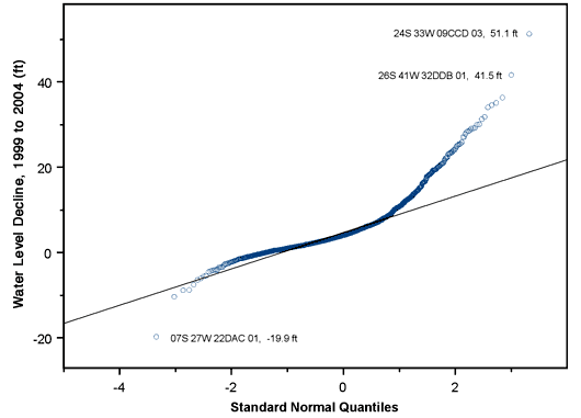
Figures 1 and 2 show histograms of the one- and five-year water level declines and Figures 3 and 4 show the corresponding normal quantile-quantile (QQ) plots. The normal QQ plots display the sorted data values plotted against the corresponding quantiles of a standard normal distribution, highlighting deviations from normality and especially the behavior in the tails of the distribution. Normally distributed data with the same mean and standard deviation as the dataset in question would fall along the straight line shown in the plot. Figures 1 and 3 emphasize that the distribution of one-year declines is sharply peaked with long tails in both directions while Figures 2 and 4 show that the five-year declines are positively skewed, with larger declines considerably more frequent than small (or negative) declines.
Figure 1--Histogram of water level declines between 2003 and 2004 campaigns.
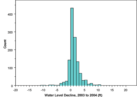
Figure 2--Histogram of water level declines between 1999 and 2004 campaigns.
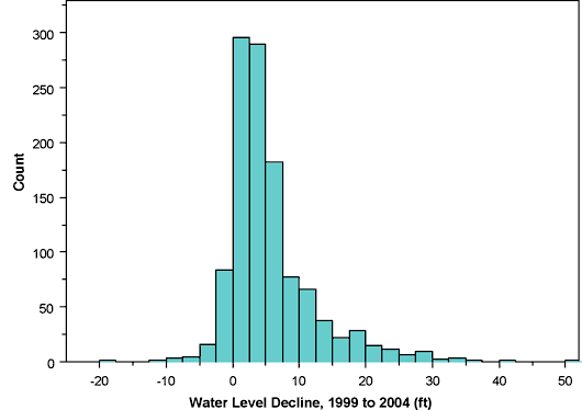
Figure 3--Normal quantile-quantile plot for one-year water level declines.
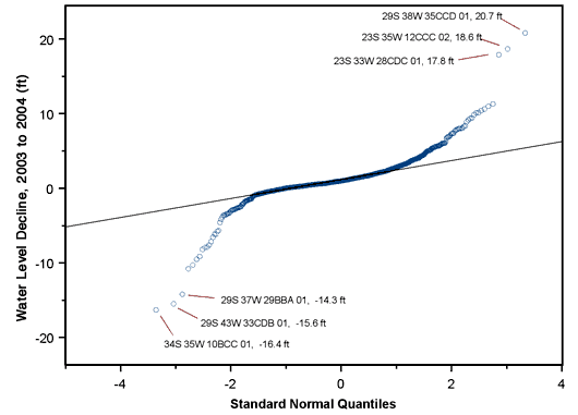
Figure 4--Normal quantile-quantile plot for five-year declines.
The most extreme values are indicated on both plots (with both the KGS ID and decline value indicated). Wells 23S 35W 12CCC 02 and 23S 33W 28CDC 01, which show up with extreme positive one-year declines, have both shown considerable fluctuation over the years. Well 34S 35W 10BCC 01, with the most extreme negative one-year decline, is a provisional well that has been measured only twice and may have been influenced by nearby pumping in 2003, leading to an anomalous apparent rebound in 2004.
For the extreme five-year declines, well 07S 27W 22DAC 01 experienced a major drop in 1999, causing it to show the largest recovery since 1999, while 24S 33W 09CCD 03 is another well that has shown considerable fluctuation over the years.
None of these values seems wholly out of line with the overall data distribution, though, and the fact that different wells exhibit the extreme one- and five-year declines seems to indicate that none of the values are due to erroneous 2004 measurements. This is borne out by further analyses.
In order to factor out the dominant influence of the spatial dependence of the water table depth, the quality control analysis focuses on the change in water level from the previous year. We performed an analysis of variance to attempt to identify unwanted sources of variation in the 2003 to 2004 water level declines in wells measured by KGS personnel in 2004. Of the 482 KGS wells located within the High Plains aquifer extent, 469 also have measurements from 2003, allowing us to compute differences between 2004 and 2003 (again, using first measurements for those wells with multiple measurements in a given year). These 469 measurements are the basis for the quality control statistical analysis.
For each measurement, several additional variables are stored in the database, including the initials of the measurer, the ease or difficulty of accessing the well, whether a weighted tape was used in the measurement, the primary use of the well, whether oil was present on the water, the chalk cut quality for the measurement, and a code indicating which aquifer(s) provide the primary source of water for the well. Ideally, none of these factors should significantly influence the depth measurement, except possibly the formations in which the well is screened.
The values taken on by these variables are as follows:
| Measurer: | BBW, BE, DRL, JMA, JTD, RB, RDM |
| Downhole Access: | Easy, Hard |
| Weighted Tape: | No Weight, Weight |
| Well Use: | H: household water supply I: irrigation S: stock water supply U: unused observation Z: animal waste disposal |
| Oil on Water: | No Oil, Oil Present |
| Chalk Cut Quality: | Excellent, Good, Fair |
| Aquifer Code (Geol.Units): |
KD: Cretaceous Dakota KJ: undifferentiated Cretaceous/Jurassic KN: Cretaceous Niobrara QA: Quaternary alluvium QAQU: Quaternary alluvium + undifferentiated Quaternary aquifers QAQUTO: Quaternary alluvium & undifferentiated + Tertiary Ogallala QATO: Quaternary Alluvium + Tertiary Ogallala QU: Quaternary undifferentiated QUTO: Quaternary undifferentiated + Tertiary Ogallala QUTOKD: Quaternary undifferentiated + Ogallala + Dakota QUTOKJ: Quaternary undifferentiated + Ogallala + Cretaceous/Jurassic TO: Tertiary Ogallala TOKD: Tertiary Ogallala + Cretaceous Dakota TOKJ: Tertiary Ogallala + Cretaceous/Jurassic |
The results for the analysis of variance are shown in Table 2
Table 2--Analysis of variance using 14 aquifer codes (Geol.Units)
| Source | Df | Sum of Sq | Mean Sq | F Value | Pr > F |
|---|---|---|---|---|---|
| Measurer | 6 | 100.1 | 16.679 | 2.3812 | 0.02828 |
| Downhole.Access | 1 | 0.3 | 0.335 | 0.0478 | 0.82705 |
| Weighted.Tape | 1 | 18.9 | 18.907 | 2.6993 | 0.10111 |
| Well.Use | 4 | 20.8 | 5.190 | 0.7410 | 0.56444 |
| Oil.On.Water | 1 | 6.1 | 6.131 | 0.8753 | 0.35000 |
| Chalk.Cut.Quality | 2 | 29.6 | 14.798 | 2.1126 | 0.12215 |
| Geol.Units | 13 | 294.8 | 22.674 | 3.2370 | 0.00011 |
| Residuals | 440 | 3082.0 | 7.004 | ||
| Residual standard error: 2.647 | |||||
Variations between geological units are significant. Variations between measurers are significant at the 5% level, but not at the 1% level. That is, the probability of obtaining a greater F value by chance, 2.8%, is less than 5% but more than 1%. Considering that there is some degree of spatial correlation between the decline values and that a given measurer covers a certain region each day, it is possible that the variation between measurers is confounded with spatial variation effects to some degree.
We also ran an analysis of variance using the five-part aquifer classification employed in the 1997 through 2002 analyses. The five-part grouping (Aq.Group) is obtained from the 14-part Geol.Units as follows:
| Aq.Group | Geol.Units | data count |
|---|---|---|
| QA (Quaternary) | QA, QAQU, QU | 38 |
| QT (Quaternary + Tertiary) | QATO, QAQUTO, QUTO | 207 |
| TO (Tertiary Ogallala) | TO | 190 |
| QK (Quaternary - Cretaceous) | QUTOKD, QUTOKJ, TOKD, TOKJ | 13 |
| KK (Cretaceous) | KD, KJ, KN | 21 |
Table 3--Analysis of variance using 5-part aquifer grouping (Aq.Group) Source
| Df | Sum of Sq | Mean Sq | F Value | Pr > F | |
|---|---|---|---|---|---|
| Measurer | 6 | 100.1 | 16.679 | 2.3678 | 0.02910 |
| Downhole.Access | 1 | 0.3 | 0.335 | 0.0475 | 0.82753 |
| Weighted.Tape | 1 | 18.9 | 18.907 | 2.6841 | 0.10206 |
| Well.Use | 4 | 20.8 | 5.190 | 0.7368 | 0.56723 |
| Oil.On.Water | 1 | 6.1 | 6.131 | 0.8704 | 0.35135 |
| Chalk.Cut.Quality | 2 | 29.6 | 14.798 | 2.1007 | 0.12357 |
| Aq.Group | 4 | 213.9 | 53.481 | 7.5924 | 0.00001 |
| Residuals | 449 | 3162.8 | 7.044 | ||
| Residual standard error: 2.654 | |||||
As shown in Table 3, grouping the 14 aquifer codes into the five-part classification results in greater significance for that factor, but does not significantly alter the results for any other factor. For this analysis, the least-squares means (expected values) of the 2003 to 2004 declines for all levels of all factors are as follows:
Global mean for 469 KGS measurements: 1.91 feet
| Measurer | |||||||
| Level | BBW | BE | DRL | JMA | JTD | RB | RDM |
| Mean | 2.69 | 1.43 | 2.20 | 1.38 | 2.17 | 2.12 | 1.61 |
| Count | 67 | 77 | 72 | 91 | 46 | 69 | 47 |
| Downhole.Access | ||
| Level | Easy | Hard |
| Mean | 1.92 | 1.84 |
| Count | 412 | 57 |
| Weighted.Tape | ||
| Level | No Weight | Weighted |
| Mean | 1.10 | 1.96 |
| Count | 26 | 443 |
| Well.Use | |||||
| Level | H | I | S | U | Z |
| Mean | 1.50 | 1.87 | 1.20 | 2.28 | 2.71 |
| Count | 6 | 374 | 14 | 73 | 2 |
| Oil.On.Water | ||
| Level | No Oil | Oil Present |
| Mean | 1.96 | 1.69 |
| Count | 385 | 84.00 |
| Chalk.Cut.Quality | |||
| Level | Excellent | Good | Fair |
| Mean | 1.92 | 2.09 | 0.69 |
| Count | 358 | 94 | 17 |
| Aq.Group | |||||
| Level | QA | QT | TO | QK | KK |
| Mean | 1.27 | 2.54 | 1.26 | 1.66 | 2.93 |
| Count | 38 | 207 | 190 | 13 | 21 |
Figures 5 and 6 show the 2003 to 2004 decline values plotted by measurer's initials and by aquifer group, the only two factors deemed significant by the analysis of variance. Clearly, there is considerable overlap between the decline values for the different measurers and nothing seems to be systematically off in the results for any one measurer. The measurer with the highest average decline (BBW, 2.69 feet) has a more uniform distribution of values, while the other measurers tend to show a somewhat greater density of lower declines. However, BBW's measurements are well within the range of all measurements. The measurer with the lowest mean (JMA, 1.38 feet) measured the most extreme negative decline, -16.4 feet, in well 34S 35W 10BCC 01, the provisional well mentioned above. Eliminating this single value brings JMA's average up to 1.57 feet, comparable to RDM's average and higher than BE's.
Figure 5--2003 to 2004 water level declines by measurer.
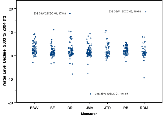
Figure 6 highlights the imbalance in number of measurements between the different aquifer groups, a factor that somewhat obscures the significance of the variation between the groups. Nevertheless, statistical tests comparing declines for the two most abundant groups, QT (wells tapping Quaternary and Tertiary aquifers) and TO (wells tapping the Tertiary Ogallala only), shows a highly significant difference between the means of these two groups. The group with the highest mean decline (wells tapping Cretaceous aquifers only) has only 21 data points, but it would not be at all surprising for these wells to exhibit substantially different behavior than those tapping younger unconsolidated and semi-consolidated formations.
Figure 6--2003 to 2004 water level declines by aquifer group.
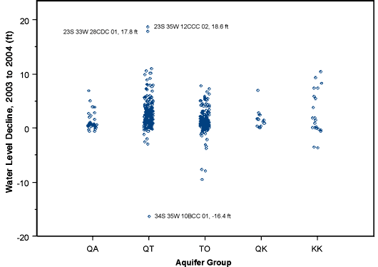
The wells with extreme values flagged in the plots are among those identified in Figure 3, the distribution plot of one-year declines for the entire set of measurements (KGS and DWR).
Examining the distribution of residuals from the expected values predicted by the ANOVA model can help to identify wells whose decline values are seriously out of line with expectations. Figure 7 shows a normal quantile-quantile plot for the residuals from the ANOVA using the five-part aquifer classification (Aq.Group), with wells showing residuals greater than 10 feet identified. These are the same three wells identified in Figures 3, 5, and 6--those with the most extreme decline values--namely,
| KGS ID | Residual |
|---|---|
| 23S35W 12CCC 02 | 16.0 ft |
| 23S 33W 28CDC 01 | 14.7 ft |
| 34S 35W 10BCC 01 | -18.6 ft |
Figure 7--Normal quantile-quantile plot for residuals from ANOVA using five-part aquifer classification.
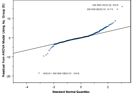
As discussed above, the first two of these wells have shown considerable fluctuation over the years and the 2003 measurement for the third may have been influenced by nearby pumping. None of these wells show up as outliers in the geostatistical analysis of water table elevations (next section), indicating that these measurements do not seem to be terribly out of line with those in nearby wells.
For the geostatistical analysis of 2004 water table elevations, we have employed the first measurements at the 1253 wells in the High Plains aquifer extent. Since the water table elevation shows a strong trend, the first task is to identify a "trend-free" direction, perpendicular to the predominant trend or roughly parallel to contours of constant elevation. The empirical variogram computed in the trend-free direction can be viewed as an approximation for the variogram of the random (but still spatially autocorrelated) component of the overall variation. The subsequent kriging analysis combines the random field variogram model with a first-order local trend model to estimate the water table elevation at all points on a regular grid.
We have computed empirical variograms for a series of azimuths, N 0° E to N 27° E in 1° increments, to search for an apparently trend-free direction. The parameters employed in the variogram computations are the same as those employed by Olea (2003), namely, a nominal lag spacing of 4 km, 25 lags overall, an azimuthal tolerance of 10° and a bandwidth of 5 km. Figure 8 shows the resulting set of directional variograms.
Figure 8--Directional variograms 2004 water table elevation, computed for N 0° E to N 27° E in 1° increments (azimuths above each plot).
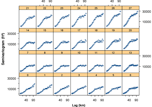
A trend-free variogram should level off to a clearly defined sill rather than continuing to rise with increasing lag. The variogram for N 12° E, the trend-free direction selected by Olea (2003) for the analysis of the 2003 measurements, looks as trend-free as any of those shown in Figure 8, so we will employ this variogram as representing the random field component of the water table elevation.
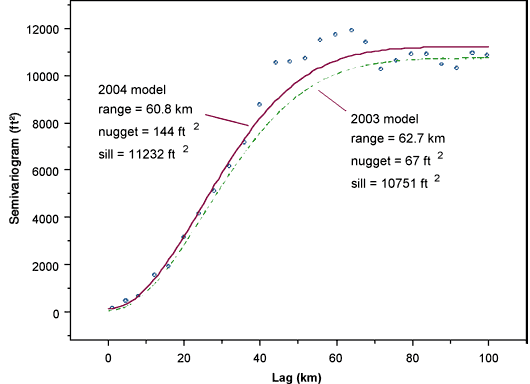
Figure 9 shows the empirical variogram for N 12° E, with two fitted Gaussian models. The 2004 model has been fitted to the empirical variogram shown using the same weighted least-squares variogram-fitting procedure (Olea, 1996) used in earlier years' analyses (Olea and Davis, 2003; Olea and Davis, 2002). The other model shown is that fitted to the 2003 data by Olea and Davis (2003). Clearly, both models are quite similar, although the 2004 model exhibits a slightly higher variance and particularly a higher nugget value. The higher variance has no significant influence on the kriged map of water table elevation but is critical to the map of the kriging standard deviation, which is used to help identify gaps in the measurement network. The impact of this difference is discussed further below.
Figure 9--Empirical variogram in direction N 12° E for 2004 water table elevations, together with Gaussian model fitted to this variogram and Gaussian model fitted to 2003 water table elevation data by Olea and Davis (2003).
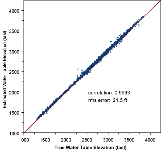
We have proceeded with a kriging analysis using the 2004 variogram model shown in Figure 9, together with a first-order trend in the geographic coordinates. Figure 10 shows the results of a crossvalidation analysis, in which each well is removed from the dataset in turn, a kriged water level is estimated at that location based on nearby measurements, and the true and estimated values are compared. Figure 10 shows the high degree of correlation and low root-mean-squared error (relative to the range of variation in water table elevation) between the estimated and actual elevations.
Figure 10--Kriging crossvalidation results for 2004 water table elevations.
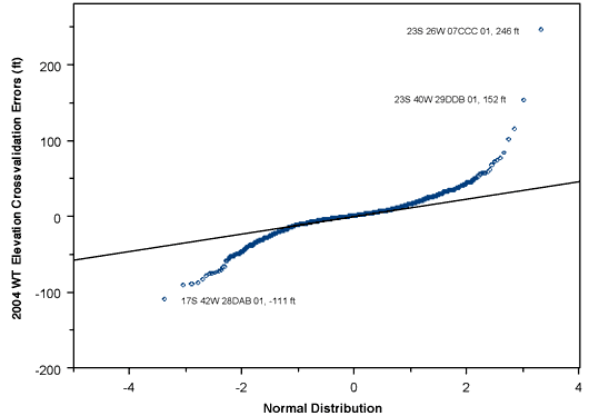
A normal quantile-quantile plot for the kriging crossvalidation errors at the KGS-measured wells is shown in Figure 11, with the three most extreme residuals flagged. A positive error means that the estimated water-table elevation is higher than the measured elevation at the well, while a negative error means the opposite. The three wells flagged are those with measurements that are most anomalous compared to those in surrounding wells, according to the kriging analysis. The two wells with the largest positive errors are both KGS wells screened in the Cretaceous Dakota aquifer. Neither of these wells showed up as a large-residual well in the quality control ANOVA described above, which would seem to indicate that these represent valid water level measurements.
Figure 11--Normal quantile-quantile plot of kriging crossvalidation errors for 2004 water table elevations.
We have performed an analysis of variance of the kriging crossvalidation errors for the wells measured by KGS personnel, against the same set of exogenous variables as used for the quality control ANOVA above. This analysis revealed a highly significant difference between crossvalidation errors for different aquifer groups and a marginally significant difference between the different values of chalk cut quality. None of the other variables were deemed significant. In particular, there were no significant differences between crossvalidation errors associated with different measurers.
Table 4--Means of kriging crossvalidation errors for 2004 water table elevations by aquifer group.
| Aq.Group | QA | QT | TO | QK | KK |
|---|---|---|---|---|---|
| Mean | 0.94 ft | -2.72 ft | -1.98 ft | 8.51 ft | 36.32 ft |
| Count | 37 | 207 | 190 | 13 | 21 |
Table 4 shows the means of the crossvalidation errors split out by aquifer group and Figure 12 is corresponding plot of error distributions. Again, the imbalance in the number of measurements between groups obscures the comparisons somewhat, but it is immediately apparent that the large mean error for wells tapping Cretaceous aquifers (group KK) is due in large part to the fact that the four largest errors are in this group. These errors indicate that the measured elevations in these wells are much lower than the elevations interpolated from the surrounding wells, perhaps indicating that the heads in Cretaceous aquifers are substantially lower than those in younger, shallower aquifers in some areas.
Figure 12--Kriging crossvalidation errors for 2004 water table elevations versus aquifer group.
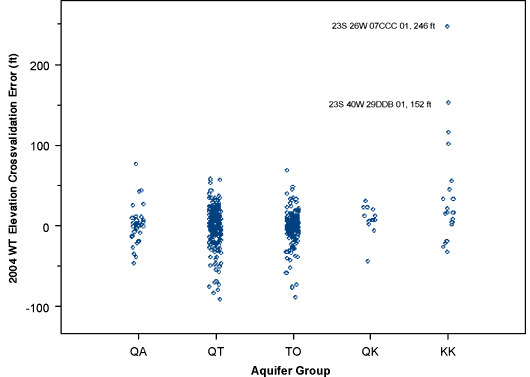
Figure 13 shows the kriged water table elevation map for the 2004 measurement campaign using the semivariogram model fit to the 2004 data (see Figure 9). The kriged map based on the lower-variance 2003 model is indistinguishable, demonstrating that the elevation estimate itself is fairly insensitive to the differences between these two models.
Figure 13--Kriged water table elevation for the 2004 measurement campaign. A larger version of this figure is available.
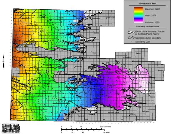
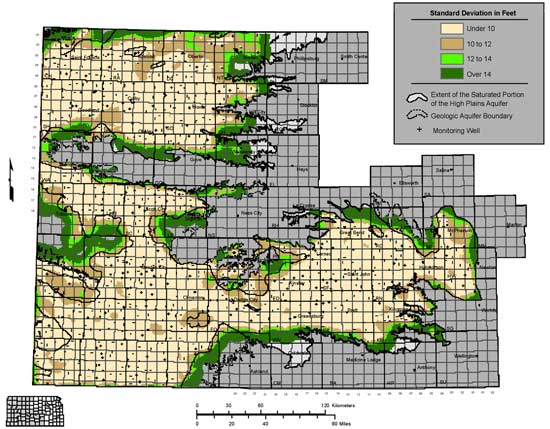
Figure 14 shows the kriging error (standard deviation) map based on the 2003 semivariogram model, with the 10-feet standard deviation contour highlighted. In past years, a ten-foot standard deviation threshold has been used to identify "holes" in the sampling network and wells in these areas were suggested for inclusion in the network, in order to achieve a kriging error of 10 feet or less throughout the region.
Figure 14--Kriging standard deviation for 2004 water table elevations using semivariogram model based on 2003 data. A larger version of this figure is available.
Using the 2004 semivariogram model, the kriging standard deviation is greater than 10 feet essentially everywhere, rendering the 10-foot threshold meaningless. However, the pattern of the kriging error depends primarily on the distribution of the wells, so that essentially the same error map is obtained from the 2004 model by scaling up the contour values appropriately, as shown in Figure 15. The contour levels employed in Figure 15 (14.4, 16.8, and 19.1 feet) represent the same percentiles of the error distribution shown on that map as the 10-, 12- and 14-foot contours do in Figure 14 (namely, 60.6%, 76.4%, and 81.9%).
Figure 15--Kriging standard deviation for 2004 water table elevations using semivariogram model based on 2004 data. A larger version of this figure is available.
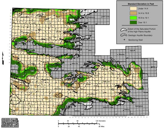
Clearly, Figures 14 and 15 convey the same information. The kriging error map is really about the distribution of well control. The exact values in the map are overly sensitive to the vagaries of variogram model fitting and also (at least to some extent) reflect the innate level of spatial variability in the water table elevations, a factor that is beyond our control. Therefore, it seems reasonable to be less concerned about the exact threshold and instead choose a contour value that helps to highlight gaps in the distribution of wells, which is achieved nicely using either the 10-foot contour on Figure 14 or the 14.4-foot contour on Figure 15. (It should be noted that some of the apparent holes in the network actually represent areas where the High Plains aquifer is absent.)
As in years past, we have determined the locations of potential gap-filling wells by overlaying a hexagonal grid on the kriging error map and looking for wells located near the center of each hexagonal bin falling over a gap as identified on the error map (Olea, 1984). The identification of network holes is described in more detail in Section 8 and Appendix A contains a listing of possible additional wells identified by this process.
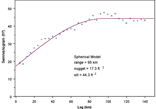
Figure 16 shows the semivariogram for the water level changes from 2003 to 2004. (The summary statistics for these changes are presented in Section 3.) Because the changes in water level do not show a strong trend, an omnidirectional semivariogram is employed. The spherical semivariogram model shown was again fitted using the weighted nonlinear least squares procedure (Olea, 1996) used for previous years' analyses (Olea and Davis, 2003). The water level declines show considerably more short-scale variability than the water levels themselves, as evidenced by the higher nugget effect relative to the overall level of variability (the sill) on this semivariogram as compared to the semivariogram for the water levels (Figure 9).
Figure 16--Omnidirectional semivariogram for changes in water level over the five-year period from 1999 to 2004.
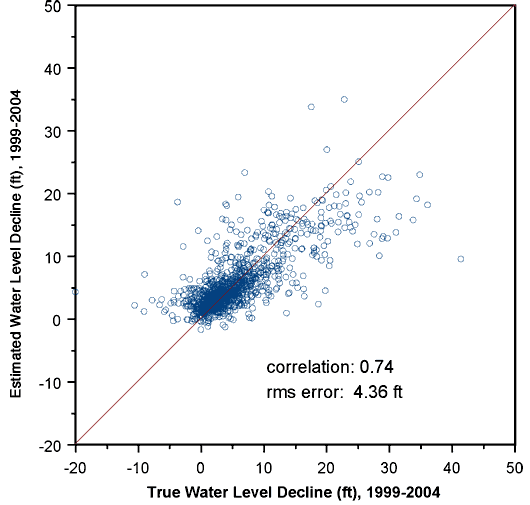
The relatively high short-scale variability in the decline values results in a significantly lower correlation between actual and estimated decline values in the kriging crossvalidation analysis (Figure 17).
Figure 17--Kriging crossvalidation results for 5-year water level changes.
The kriged five-year declines are shown in Figure 18. The corresponding kriging standard deviation map is shown in Figure 19.
Figure 18--Water level changes for the five-year interval from 1999 to 2004. A larger version of this figure is available.
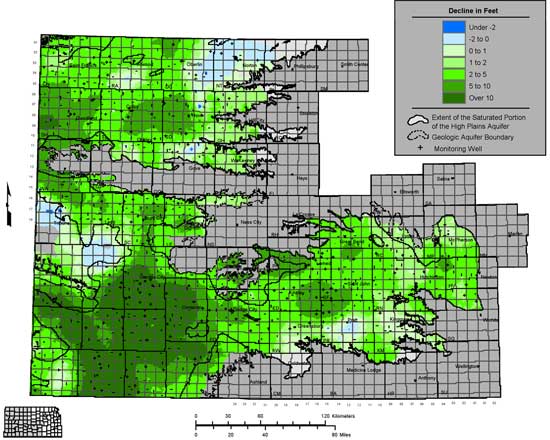
Figure 19--Kriging standard deviation for the five-year water level changes from 1999 to 2004. A larger version of this figure is available.
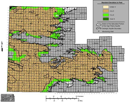
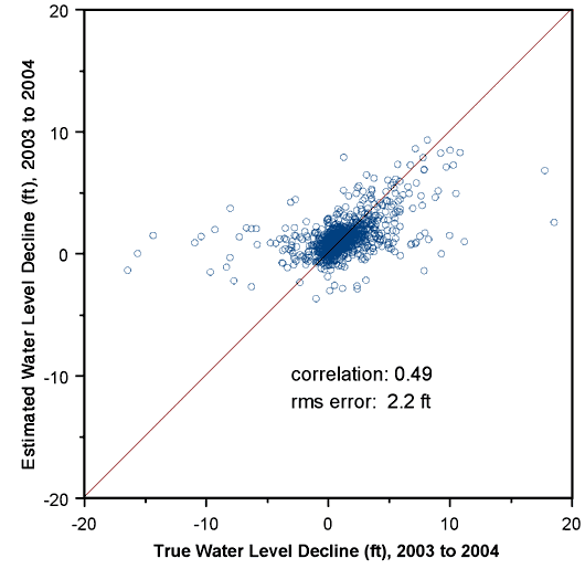
Figure 20 shows the omnidirectional semivariogram for the water level changes from 2003 to 2004, along with the fitted semivariogram model. These declines show an even higher relative level of short-scale variation, leading to decreased accuracy in the kriging estimates (Figure 21). Now the crossvalidation analysis leads to a correlation of only 0.49 between the measured and estimated water-level changes at the wells.
Figure 20--Omnidirectional semivariogram for changes in water level between 2003 and 2004 measurement campaigns.
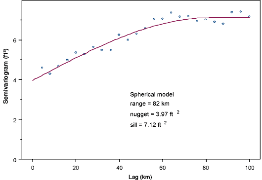
Figure 21--Kriging crossvalidation results for changes in water level between 2003 and 2004.
As with the crossvalidation analysis of water table elevations, it is possible to compute the difference, or kriging error, between the estimated and true water-level changes at each well. It is instructive to perform an analysis of variance of these kriging errors (at wells measured by KGS personnel) against the same exogenous variables employed in the quality control analysis described in Section 4. By looking at the kriging errors, which indicate the discrepancy between the decline measurement at each well relative to those in surrounding wells, we are essentially factoring out the spatial dependence that would possibly be confounded with some of the factors in the ANOVA of the decline values themselves. The ANOVA of the kriging residuals (Table 5) reveals no significant dependence on any of the exogenous variables, indicating that none of these factors seems to induce any systematic deviation in water level decline measurements when compared to surrounding wells. The lack of systematic dependence of the kriging errors on any of the exogenous variables is a strong indication of the quality of the measurement process.
Table 5--Analysis of variance of kriging errors for 2003 to 2004 water level changes.
| Source | Df | Sum of Sq | Mean Sq | F Value | Pr > F |
|---|---|---|---|---|---|
| Measurer | 6 | 8.851 | 1.475 | 0.3137 | 0.9298 |
| Downhole.Access | 1 | 6.464 | 6.464 | 1.3746 | 0.2417 |
| Weighted.Tape | 1 | 0.035 | 0.035 | 0.0074 | 0.9314 |
| Well.Use | 4 | 7.783 | 1.946 | 0.4138 | 0.7987 |
| Oil.On.Water | 1 | 9.121 | 9.121 | 1.9394 | 0.1644 |
| Chalk.Cut.Quality | 2 | 9.530 | 4.765 | 1.0132 | 0.3639 |
| Aq.Group | 4 | 14.341 | 3.585 | 0.7624 | 0.5502 |
| Residuals | 449 | 2111.574 | 4.703 | ||
| Residual standard error: 2.169 | |||||
Figure 22 is the kriged map of water level declines from 2003 to 2004 and Figure 23 is the corresponding standard deviation map. The standard deviation map shows that the kriging error in many locations is of the same magnitude as the estimated water level changes. Nevertheless, the pattern of declines is fairly coherent and also consistent with the declines over the interval from 1999 to 2004. One notable exception appears in eastern Stevens County just north of the Kansas-Oklahoma border. This is an area of strong decline over the five-year period but experienced an increase in water level between 2003 and 2004.
Figure 22--Water level changes from 2003 to 2004. A larger version of this figure is available.
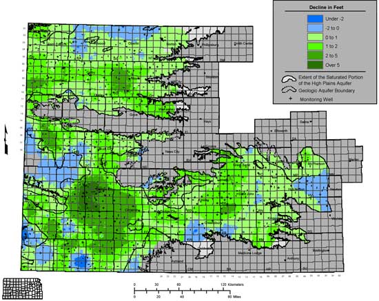
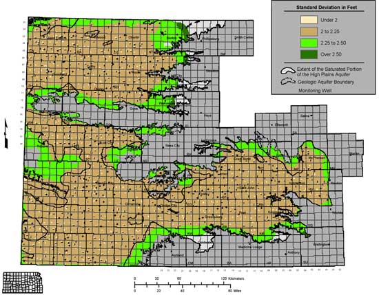
Figure 23--Kriging standard deviation for the 2003 to 2004 water level changes. A larger version of this figure is available.
Both kriging error maps (standard deviation) shown in Figure 14 and Figure 15 indicate areas of the High Plains aquifer where suitable well control, in terms of spatial distribution, is lacking. These areas are referred to as network "holes" and are caused by absent depth to water measurements in those locations. A common reason holes occur is that a monitoring well becomes un-measurable or has been permanently removed or capped. In these cases, a new replacement well is needed. In other cases, a network hole will occur because an existing monitoring well could not be access and could not be measured for that year. For example, the well was pumping or physical access to the well was not possible and thus it was not measured. In these cases where the lack of a measurement is thought to be temporary in nature, a replacement well is not found. If a measurement can not be obtained for three years, then a replacement well will be identified.
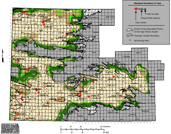
Replacement wells are found by placing a hexagonal grid over the kriging error maps (Olea, 1984). Each hexagon cell is roughly 16 square miles in size and the goal is to identify a replacement well at the center of the grid. The grid center is also referred to as the hole center. Figure 24 shows the identified network hole centers related to the 2004 measurement campaign.
Figure 24--Network holes from the 2004 measurement campaign. A larger version of this figure is available.
For each hole center, a list of well candidates are selected from the three major ground water well inventories in Kansas. Those databases specifically are the Water Well Completion Records (WWC5), the Water Information Storage and Retrieval Database (WIZARD), and the Water Information Management and Analysis System (WIMAS). Wells within 1 to 2 miles, and if needed, 3 miles from the hole centers are reviewed for potential inclusion in the monitoring network. The preferred replacement well is a true observation well or newly constructed irrigation well. Once the list of well candidates has been selected, the associated landowners are contacted for permission to measure the well and include it in this voluntary program. The list of well replacement candidates are shown in Appendix A.
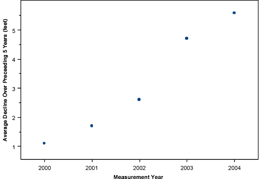
The statistical quality control analysis for the 2004 campaign reveals no significant sources of unwanted variation in the water level measurements, testifying to the quality of the measurement procedures. The level of spatial variability in water table elevation indicated by the variogram model fit to the 2004 data precludes the use of a 10-foot kriging standard deviation threshold in the identification of gaps in the measurement network, but a map based on an appropriately scaled-up threshold yields essentially the same information. The mean water level decline between the 2003 and 2004 measurement campaigns was 1.18 feet. This is somewhat less than that over the previous year (1.9 feet), but still higher than the average decline rate over the five years from 1999 to 2004 (1.12 feet/year). The pattern of decline between 2003 and 2004 was largely consistent with that for previous years, although a significant reversal in trend is apparent in eastern Stevens County, in the southwest corner of the state. The average decline between 1999 and 2004, 5.58 feet, is higher than that for the previous five-year interval (4.7 feet between 1998 and 2003), continuing a steady increase in five-year decline rates over the past several years (Figure 25).
Figure 25--Average water level declines over five-year intervals preceding each measurement year.
Davis, J. C., 2003, Statistical quality control analysis for year 2003 water well measurements, Kansas Geological Survey Open File Report 2003-8, 19 p. [Available Online]
Davis, J. C., 2001, Statistical quality control for year 2001 water well measurements, Kansas Geological Survey Open File Report 2001-2, 23 p. [Available Online]
Deutsch, C. V., and A. G. Journel, 1998, GSLIB: Geostatistical Software Library and User's Guide, Second Edition, Oxford University Press, New York, 369 p.
Olea, R. A., and J. C. Davis, 2003, Geostatistical analysis and mapping of water-table elevations in the High Plains aquifer of Kansas after the 2003 monitoring season, Kansas Geological Survey Open File Report 2003-13, 22 p, 11 plates. [Available Online]
Olea, R. A., and J. C. Davis, 2002, Geostatistical analysis and mapping for year 2002 water levels in the High Plains aquifer of Kansas, Kansas Geological Survey Open File Report 2002-14, 34 p, 16 plates. [Available Online]
Olea, R. A., 1984, Sampling design optimization for spatial functions, Mathematical Geology, vol. 16, no. 4, p. 369-392.
Olea, R. A., 1996, XVAN: A computer program for the analysis of spatial estimation errors: Computers & Geosciences, v. 22, no. 4, p. 445-448.
Next Page: Appendix A--List of suggested wells for filling monitoring networkholes
Kansas Geological Survey, Water Level CD-ROM
Send comments and/or suggestions to webadmin@kgs.ku.edu
Updated Dec. 30, 2004
Available online at URL = http://www.kgs.ku.edu/Magellan/WaterLevels/CD/Reports/OFR04_57/rep00.htm