![]()
![]()
![]()
Kansas Geological Survey, Open-file Report 2000-62
Part of the Well Tests for Site Characterization Project
also part of the Direct Push Methods for Hydrostratigraphic Characterization Project
by James J. Butler, Jr., Alyssa A. Lanier, John M. Healey, and Stephen M. Sellwood
Kansas Geological Survey, University of Kansas
and
Wesley McCall and Elizabeth Garnett
Geoprobe Systems, Inc.
KGS Open File Report 2000-62
Prepared in conjunction with a presentation by Lanier et al. at the
Geological Society of America Annual Meeting and Exposition, Reno, NV
November 14, 2000
A large body of research has found that spatial variations in hydraulic conductivity (K) play an important role in determining how a contaminant plume will move in an aquifer. Unfortunately, the acquisition of information about spatial variations in K on a scale of relevance for contaminant transport investigations has proven to be a difficult task. A new direct-push-based method has been developed in an attempt to make information about spatial variations in hydraulic conductivity easier to acquire (McCall et al., 2000). This approach involves performing series of slug tests in direct-push rods as the rods are driven progressively deeper into the formation. The method has been designed so that the screened interval is only exposed to the formation during the slug tests. Clay and silt buildup associated with driving an unshielded screen through a heterogeneous sequence is thus avoided, significantly reducing the amount of well development. This approach was evaluated at an extensively studied research site in the Kansas River floodplain. A series of profiles were collected through the site's 10.7 meter thick sand and gravel aquifer near two existing fully screened wells. Profiles of K versus depth had previously been obtained at these wells using multilevel slug tests, the dipole flow probe, and borehole flowmeter surveys. The direct-push hydraulic profiling results are in good agreement with K estimates from these two wells and provide a rarely obtained view of the nature of hydrostratigraphic continuity at various levels within an aquifer. This field investigation demonstrates that direct-push hydraulic profiling enables valuable information about spatial variations in hydraulic conductivity to be obtained in an efficient manner and without the need for permanent wells.
The ease of access to the subsurface that is offered by direct-push technology in unconsolidated formations can be exploited for hydraulic testing applications. We have shown previously that hydraulic tests can be performed with direct-push equipment to obtain estimates of hydraulic conductivity (K) that are in very good agreement with the results of tests in conventional wells (Butler et al., in review). That favorable comparison was obtained using a shielded screen tool at the lower end of a string of direct-push probe rods. The approach involved driving the probe rods to a specified depth, unshielding the screen, developing the test interval, and performing a series of slug tests. The probe rods must be removed from the hole and the shielded screen reset prior to proceeding to a deeper interval. This need to continually remove the probe rods and reset the screen shield after testing each interval limits the potential of the approach for use in a continuous profiling mode.
Hinsby et al. (1992) proposed a continuous profiling method using an unshielded screen and presented results from a field investigation in a very homogeneous sand unit. Although their approach appears reasonable in homogeneous formations, we have found that driving an unshielded screen through a heterogeneous sequence will often lead to a buildup of low-K material that can be very difficult to remove with standard development procedures. We have recently developed a new hydraulic profiling method (McCall et al., 2000) in an attempt to merge the single-level shielded screen technique with the continuous profiling approach of Hinsby et al. (1992). This new method allows near-continuous profiling without exposing the screen to the formation during driving and without requiring the removal of the entire rod string from the hole prior to moving to a deeper interval. In this report, we will present an initial application of the new profiling method.
The procedures described in this report were evaluated at an experimental research site of the Kansas Geological Survey. This site, the Geohydrologic Experimental and Monitoring Site (GEMS), is located in the floodplain of the Kansas River just north of Lawrence, Kansas (Figures 1-2). The shallow subsurface at the site consists of 21+ meters (70 ft) of unconsolidated Holocene sediments of the Kansas River alluvium that overlie and are adjacent to materials of Pennsylvanian and Pleistocene age. Figure 3 displays a cross-sectional view of the shallow subsurface at GEMS with electrical conductivity logging data obtained using a direct-push unit (see Figures 4-5 and Butler et al. (1999a)), and a geologic interpretation from core and logging data. The heterogeneous alluvial facies assemblage at GEMS essentially consists of 10.7 meters (35 ft) of primarily clay and silt overlying 10.7 meters of sand and gravel. For the last decade, GEMS has been the site of extensive research on flow and transport in heterogeneous formations (e.g., McElwee et al., 1991; Butler et al., 1998, 1999a,b). This previous work enables the procedures discussed here to be evaluated in a relatively controlled field setting.
Figure 1. Location map for GEMS.
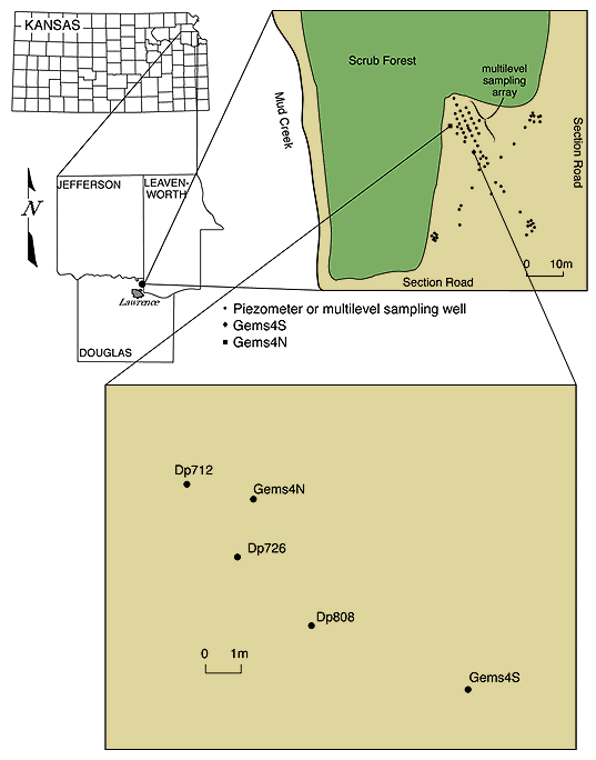
Figure 2. Photo of GEMS well array and research setup.
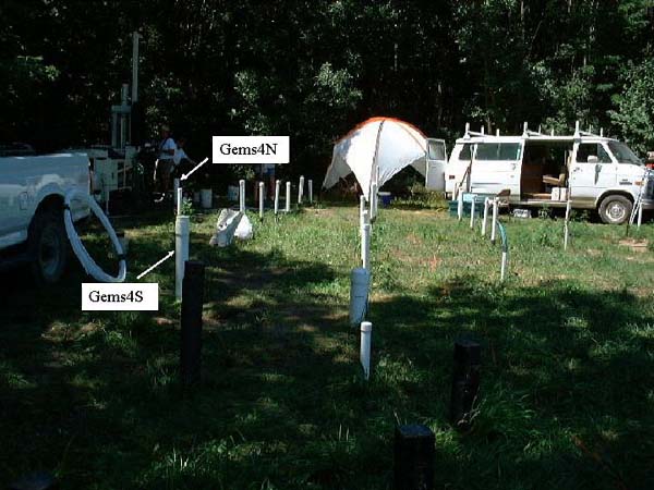
Figure 3. Generalized GEMS stratigraphy with example electrical conductivity log.
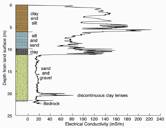
Figure 4. Photo showing direct-push unit and electrical-conductivity logging system.
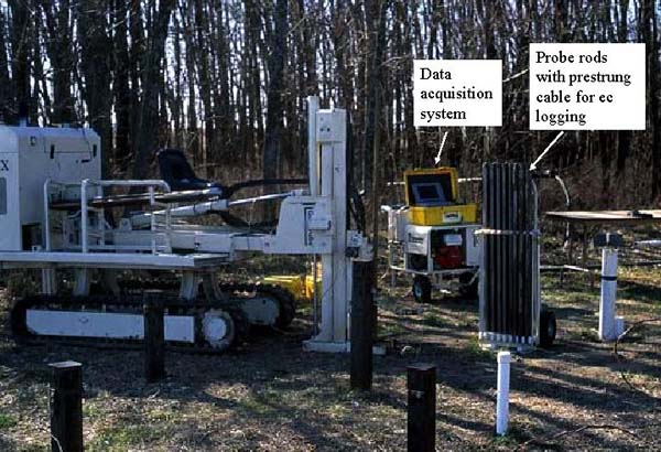
Figure 5. Schematic of direct-push electrical-conductivity logging and example log.
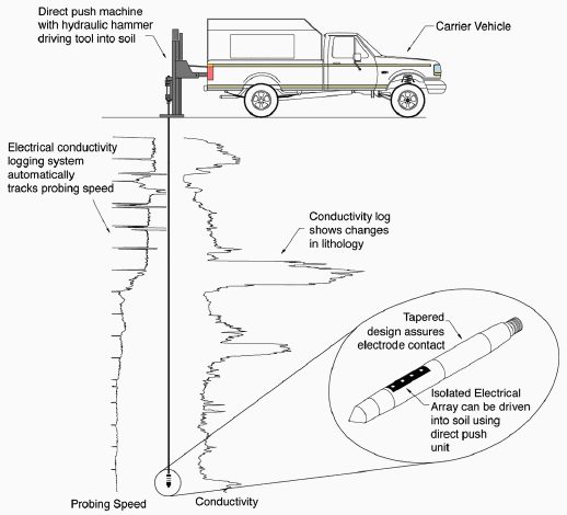
Figure 6. Schematic of profiling process.
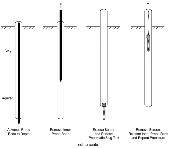
Figure 7. Photo of profiling equipment.
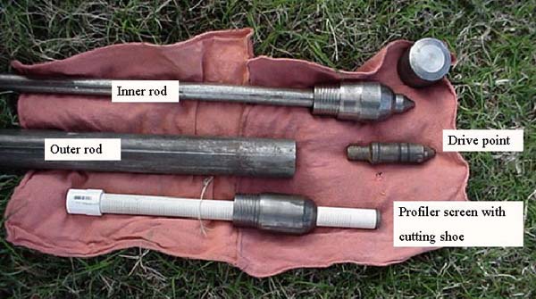
Figure 8. Schematic of placement procedure.
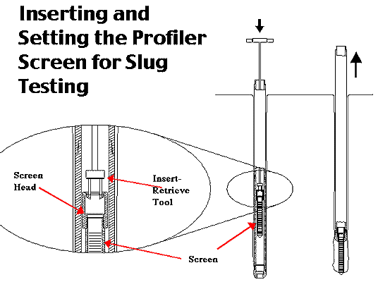
Figure 9. Photo showing development of test interval (suction pump in lower left hand corner).
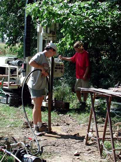
Figure 10. Attaching pneumatic well head prior to slug test.
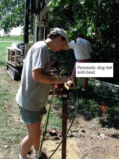
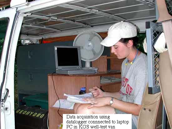
Figure 11. Acquiring slug-test data.
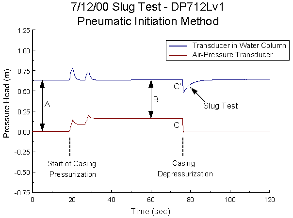
All the slug tests described in this report were initiated pneumatically, and head data were collected using pressure transducers connected to a datalogger. Figure 12 lists the major steps involved with the pneumatic initiation of a slug test, Figure 13 is a schematic of the direct-push adaptation of the pneumatic approach, and Figure 14 is an example of a test initiated with this method. As described in Butler (1997), the pneumatic method involves pressurizing the air column above the water by the injection of compressed air or nitrogen gas. This pressurization produces a depression of the water level as water is driven out of the pipe in response to the increased air pressure. The water level drops until the magnitude of the water-level change (A-B on Figure 14) is equal to the increase in the pressure head of the air column (C on Figure 14). At that point, the well has returned to equilibrium conditions (a transducer in the water column has the same reading as prior to pressurization) and the test can be initiated by rapidly depressurizing the air column. Butler (1997) and Butler et al. (in review) discuss how the C'/C ratio provides valuable information about the validity of several assumptions commonly invoked for the analysis of slug-test data.
Figure 12. Steps involved with the pneumatic initiation of a slug test.
Figure 13. Schematic of the setup for the pneumatic initiation method.
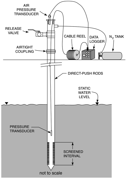
Figure 14. Example of a slug test initiated with the pneumatic method.
All the tests conducted in this study were analyzed with the high-K extension of the Hvorslev (1951) method (this extension designated as the linearized variant of the McElwee et al. model in Butler (1997)). The major steps in this analysis are outlined in Figure 15, where rc is casing radius, rw is screen radius, and b is screen length.
Figure 15. Steps used in slug-test analysis.
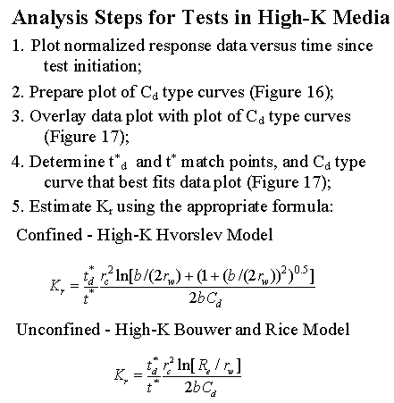
Figure 16. Type curves for slug tests in high-K media.
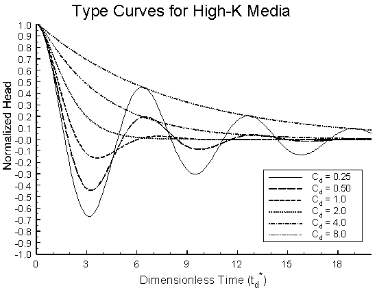
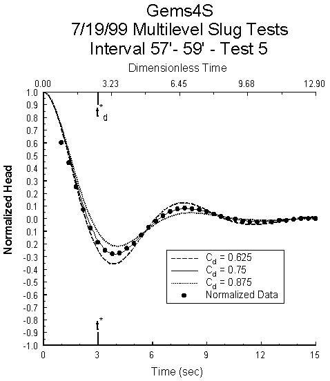
Figure 17. Example analysis.
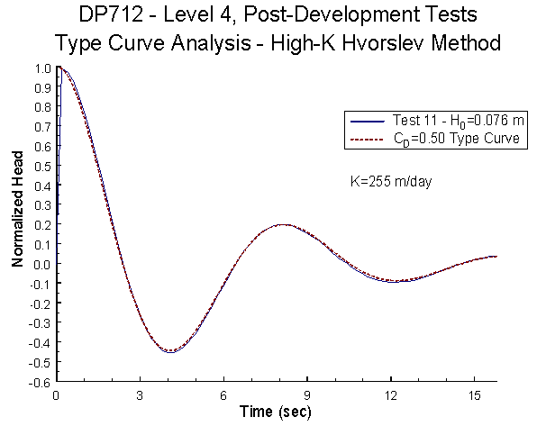
Butler et al. (1996) and Butler (1997) state that a dependence on initial displacement (H0) has often been observed in slug tests in formations of very high hydraulic conductivity. This dependence is assumed negligible in the high-K extension of the Hvorslev model. The validity of that assumption was verified for each test interval by the performance of repeat tests in which the initial displacement was varied by a factor of three or more (see Figures 18-19). When there was a negligible dependence on the initial displacement (Figure 18), a test with a relatively large H0 was used in the analysis to maximize the signal-to-noise ratio (Figure 20). In cases where test responses depended on the initial displacement, the test with the largest H0 for which this dependence could be neglected was used in the analysis (Figure 21).
Figure 18. Tests from an interval in which there was a negligible dependence on initial displacement.
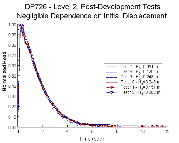
Figure 19. Tests from an interval in which there was a significant dependence on initial displacement.
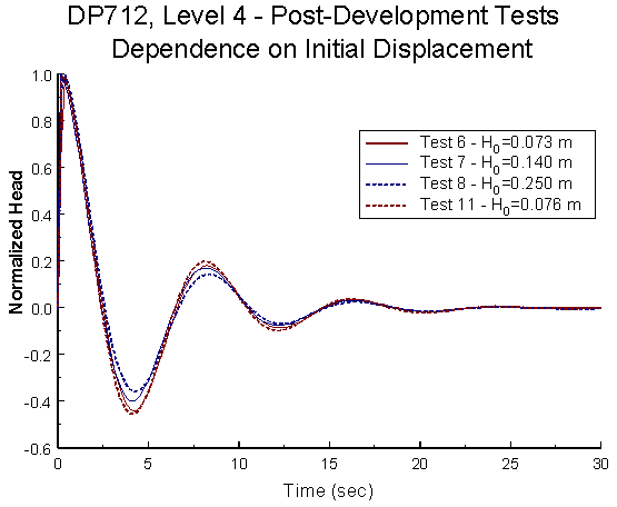
Figure 20. Type curve analysis for test 9 of Figure 18.
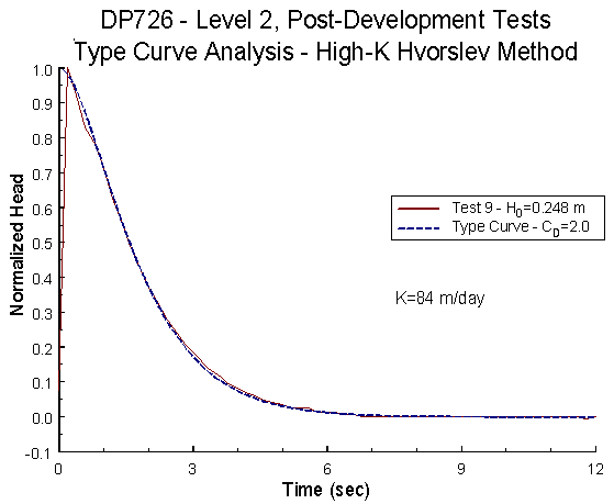
Figure 21. Type curve analysis for test 11 of Figure 19.
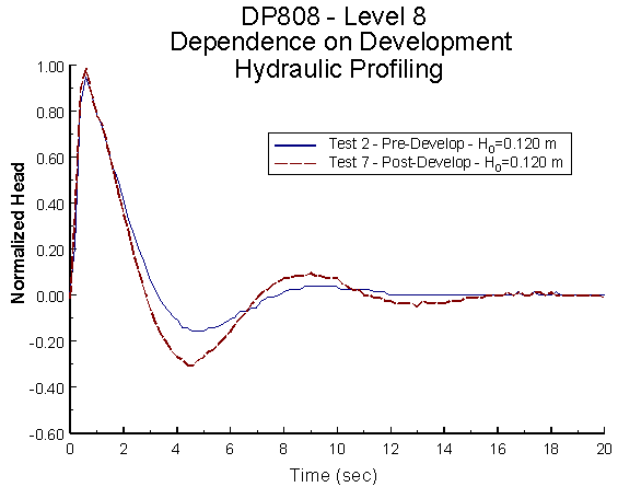
A major advantage of the hydraulic profiling approach is that the screen is not exposed to the formation while the probe rods are advanced. Thus, the need for and intensity of well development activities are considerably less than when an unshielded screen is driven through a heterogeneous sequence (compare Figures 22 and 23). A two-stage development procedure was used for the hydraulic profiling application described here. The test interval was first subjected to several minutes of pneumatic surging using the pneumatic slug-test well-head (Figure 13). The air column above the water was rapidly pressurized and depressurized using pressure heads of up to one meter. The installation was then pumped using a suction or inertial pump for approximately 15-20 minutes (Figure 9). The comparisons reported in the following section demonstrate the effectiveness of this development procedure.
Figure 22. Pre- vs. post-development comparison for profiling using unshielded screen.
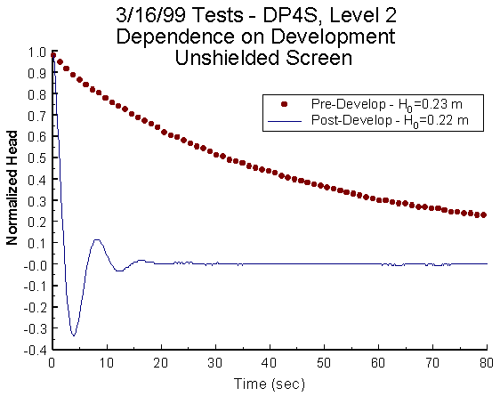
Figure 23. Pre- vs. post-development comparison for profiling using shielded screen.
The results from the hydraulic profiling were compared to results from tests performed using two conventional wells (Gems4N and Gems4S--see Figure 1; 0.102 m (4") ID; installed with hollow-stem augers). These wells, which are fully screened across the sand and gravel, have been the focus of research on techniques for estimation of vertical variations in K (e.g., Butler et al., 1998). Figure 24 presents K estimates from a series of multilevel slug tests performed in these wells in the summer of 1999 and estimates obtained two years earlier using the dipole flow probe of Zlotnik and Zurbuchen (1998--see Butler et al., 1998). The excellent agreement between K estimates obtained with completely different approaches enables the profiles of Figure 24 to be considered as standards to which the hydraulic profiling results can be compared. The superposition of the electrical conductivity log on Figure 24 helps explain some of the variability in K observed at the two wells.
Figure 24. Comparison of K estimates from multilevel slug tests and dipole flow tests.
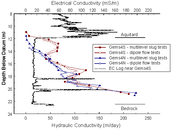
Figure 25 displays a comparison between Gems4N and the hydraulic profile at DP712. The agreement is very good at all four levels tested at DP712 (<12% difference in worst case). Figure 26 presents results from all three profiles (eight levels tested at both DP726 and DP808). Heterogeneity coupled with differences in the length and placement of the test interval produced significant differences between the hydraulic profiling results and the K estimates from Gems4N and Gems4S at several levels. For example, DP726 and DP808 indicate a low-K zone around 19 meters below datum, which is also reflected in the electrical conductivity log of Figure 24. Although this zone appears to be relatively continuous from the results of the hydraulic profiling and the electrical conductivity logging, its thickness must be much less than one meter or it would have had a greater impact on the multilevel slug tests. Similarly, at other depths, the hydraulic profiling results indicate the existence of thin high-K intervals (e.g., DP726 and DP808 at 15 meters below datum) that have little impact on the multilevel slug tests.
Figure 25. Comparison of K estimates from Gems4N and DP712.
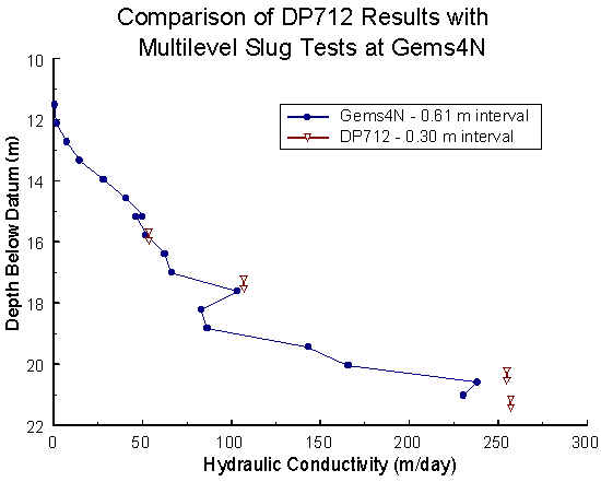
Figure 26. Comparison of K estimates from all three hydraulic profiles and Gems4N and Gems4S.
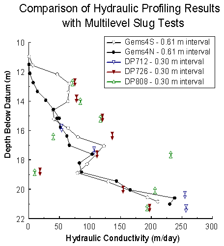
Figures 25 and 26 demonstrate the potential of the hydraulic profiling approach. Valuable information about K variations can be obtained for specific zones of interest without the need for permanent wells. The results of this initial field application indicate that hydraulic profiling can be an important tool for ascertaining the nature of hydrostratigraphic continuity at various levels within an aquifer.
The major advantages and disadvantages of the hydraulic profiling method are as follows:
Major Advantages:
Major Disadvantages:
Current work is directed at modifying the approach to reduce the impact of these limitations.
Alyssa Lanier and Steven Sellwood were the Summer 2000 participants in the Applied Geohydrology Summer Research Assistantship program of the Kansas Geological Survey. This program is open to graduate and upper-level undergraduate students at any university with an interest in learning more about recent developments in hydrogeological field methods. A portion of Alyssa Lanier's financial support was provided by the Field Research Mentoring program of the American Association of State Geologists. Additional support was provided by a grant from the Kansas Water Resources Research Institute.
Butler, J.J., Jr. 1997. The Design, Performance, and Analysis of Slug Tests. Boca Raton, Lewis Publishers.
Butler, J.J., Jr., J.M. Healey, W. McCall, E.J. Garnett, and S.P. Loheide, II. Hydraulic tests with direct-push equipment. Ground Water: in review.
Butler, J.J., Jr., J.M. Healey, L. Zheng, W. McCall, and M.K. Schulmeister. 1999a. Hydrostratigraphic characterization of unconsolidated alluvium with direct-push sensor technology (abstract). GSA 1999 Annual Meeting Abstracts with Program. v. 31, no. 7: A350 (full report (Kansas Geological Survey Open-File Rept. 99-40) available at www.kgs.ku.edu/Hydro/Publications/OFR99_40/index.html).
Butler, J.J., Jr., J.M. Healey, V.A. Zlotnik, and B.R. Zurbuchen. 1998. The dipole flow test for site characterization: Some practical considerations (abstract). EOS 79, no. 17: S153 (full report (Kansas Geological Survey Open-File Rept. 98-20) available at www.kgs.ku.edu/Hydro/Publications/OFR98_20/index.html).
Butler, J.J., Jr., C.D. McElwee, and G.C. Bohling. 1999b. Pumping tests in networks of multilevel sampling wells: Motivation and methodology. Water Resour. Res. 35, no. 11: 3553-3560.
Butler, J.J., Jr., C.D. McElwee, and W.Z. Liu. 1996. Improving the reliability of parameter estimates obtained from slug tests. Ground Water 34, no. 3: 480-490.
Hinsby, K., P.L. Bjerg, L.J. Andersen, B. Skov, and E.V. Clausen. 1992. A mini slug test method for determination of a local hydraulic conductivity of an unconfined sandy aquifer. Jour. of Hydrology 136: 87-106.
Hvorslev, M.J. 1951. Time lag and soil permeability in ground-water observations. Bull no. 36. Waterways Exper. Sta., Corps of Engrs., U.S. Army.
McCall, W., E.J. Garnett, J.J. Butler, Jr., and J.M. Healey. 2000. A dual tube direct push method for vertical profiling of hydraulic conductivity in unconsolidated formations. GSA 2000 Annual Meeting Abstracts with Program: p.A-522.
McElwee, C.D., J.J. Butler, Jr., and J.M. Healey. 1991. A new sampling system for obtaining relatively undisturbed cores of unconsolidated coarse sand and gravel. Ground Water Monitoring Review 11, no. 3: 182-191.
Zlotnik, V.A., and B.R. Zurbuchen. 1998. Dipole probe: Design and field applications of a single-borehole device for measurements of vertical variations in hydraulic conductivity. Ground Water 36, no. 6: 884-893.
Kansas Geological Survey, Geohydrology
Placed online November 2000
Comments to webadmin@kgs.ku.edu
The URL for this page is HTTP://www.kgs.ku.edu/Hydro/Publications/OFR00_62/index.html