Kansas Geological Survey, Open-file Report 2006-20
by
Geoffrey C. Bohling and Blake B. Wilson
KGS Open File Report 2006-20
July 2006
The High Plains aquifer is the primary source of water for the High Plains region of western and south-central Kansas. Some water is also withdrawn from bedrock units, primarily Cretaceous strata, in this region. The Kansas Geological Survey (KGS) and the Kansas Department of Agriculture's Division of Water Resources (DWR) measure water levels in aquifers of the High Plains on an annual basis in a network of over 1300 wells, in order to assist in the management of this vital resource. This report presents the statistical quality control analysis for the High Plains region in Kansas based on data from the 2006 water-level measurement campaign along with geostatistical analyses of the 2006 water-table elevations and water-level changes for the one-year and five-year periods preceding the 2006 measurements. In addition, it also reports summary information regarding water-level changes over the decade between the 1996 and 2006 measurement campaigns. The range of dates for the 2006 measurements was from December 9, 2005, to February 27, 2006, but the vast majority of measurements were made in early January 2006. Thus, these will be referred to as the "January 2006" or simply "2006" measurements and measurements from earlier years will be represented similarly.
Throughout this report we refer to water-level declines, with a positive decline meaning an increase in depth to water from the land surface (or decrease in water-table elevation) and a negative decline meaning a decrease in depth to water from the land surface (increase in water-table elevation). Water levels are measured in the winter so that the water table (or potentiometric surface) will have had a chance to recover from the more transient and localized effects of pumping for irrigation. The measurements are presumed to represent a new "static" water level, with the difference from the previous year's measurements representing the net loss or gain of saturated thickness over the preceding year. The difference in depth to water between the January 2006 and January 2005 measurements represents the water level decline for 2005.
The overall average water-level decline in the High Plains region over the 2005 calendar year was 0.57 feet, somewhat more than the average decline over 2004 (0.15 feet) but less than the average annual decline rate over the five years since the 2001 measurement campaign (approximately 0.98 feet/year).
Note that the current measurement approach, with responsibility divided primarily between the DWR and the KGS, began with the 1997 measurement campaign. Although the January 2006 measurements represent the tenth such campaign, they represent only nine years of water level change relative to January 1997, when current protocols were initiated. This report will contain a preliminary assessment of decadal changes, using the (nominal) January 1996 measurements as a reference point. However, protocols for the 1996 campaign were substantially different, so comparisons may not be completely accurate. We plan on preparing a more extensive decadal water level report next year, following the 2007 measurement campaign.
We would like to thank the external reviewer of this manuscript, Wayne Bossert, Manager, Northwest Kansas Groundwater Management District Number 4, and the internal (KGS) reviewers, Rex Buchanan and Don Whittemore, for their helpful suggestions for improving this report.
The SQL query shown in Listing 1 was used to extract water-level measurements for the 2006 campaign from the Kansas Geological Survey's Water Information Storage and Retrieval Database (WIZARD). Natively, WIZARD is stored in an Oracle relational database schema storing depth to water information across the state. To facilitate SQL queries for analysis, the official network wells targeted each year for the water level measurement campaigns have been identified into Oracle "Views". The view BWILSON.WIZARD_NETWORK_WELLS represents the individual well locations where measurements are attempted each year and the view BWILSON.WIZARD_NETWORK_WELLS_WL accesses the corresponding water level measurements for those sites.
Listing 1. SQL query for extracting 2006 water-level measurements from WIZARD.
select
    bwilson.wizard_network_wells_wl.*,
    bwilson.wizard_network_wells.land_surface_altitude as surf_elev,
    bwilson.wizard_network_wells.latitude as latitude,
    bwilson.wizard_network_wells.longitude as longitude,
    bwilson.wizard_network_wells.well_access,
    bwilson.wizard_network_wells.downhole_access,
    bwilson.wizard_network_wells.use_of_water_primary,
    bwilson.wizard_network_wells.geological_unit1 ||
    bwilson.wizard_network_wells.geological_unit2 ||
    bwilson.wizard_network_wells.geological_unit3 as geol_units,
    bwilson.wizard_network_wells.local_well_number as kgs_id,
    bwilson.wizard_network_wells.other_identifier as AnnProv
  from
    bwilson.wizard_network_wells_wl, bwilson.wizard_network_wells
  where
    bwilson.wizard_network_wells_wl.usgs_id =
         bwilson.wizard_network_wells.usgs_id and
    bwilson.wizard_network_wells_wl.depth_to_water is not null and
    (bwilson.wizard_network_wells_wl.agency = 'KGS' or
        bwilson.wizard_network_wells_wl.agency = 'DWR' ) and
    bwilson.wizard_network_wells_wl.measurement_date_and_time >=
                '01-Dec-2005' and
    bwilson.wizard_network_wells_wl.measurement_date_and_time <=
                '28-Feb-2006'
  order by
    bwilson.wizard_network_wells_wl.usgs_id,
    bwilson.wizard_network_wells_wl.measurement_date_and_time
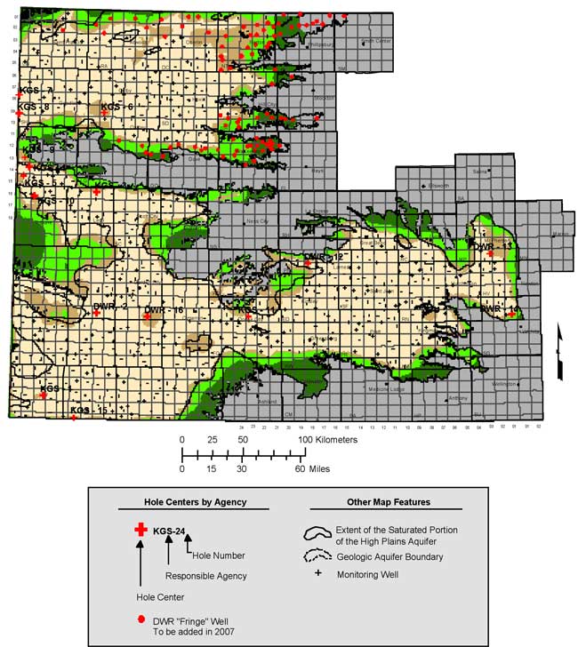
The query yields 1373 measurements from 1306 distinct wells, with measurement dates ranging from December 9, 2005, to February 27, 2006. Of these wells, 1266 are located within the geographic boundaries demarking the saturated extent of the High Plains aquifer, 712 of them measured by DWR staff and 554 by KGS staff. Figure 1 shows the distribution of responsibility between the two agencies. The KGS is now primarily responsible for measuring wells in the western and southwestern portions of the network, whereas the DWR is responsible for the central and eastern portions.
Figure 1. Wells measured and responsible agency in 2006.
The wells within the extent of the High Plains aquifer are screened primarily in that aquifer but also include some wells screened in alluvial aquifers or in underlying bedrock. WIZARD contains fields identifying up to three different geologic units tapped by each well and the SQL query extracts this unit information, concatenated in the single variable "geol_units". The query also extracts location data (latitude, longitude, and surface elevation) along with the additional variables used in the statistical quality control analysis. Similar queries were used to extract data from the 2005 and 2001 measurement campaigns for the sake of computing 1-year and 5-year water-level changes.
Repeat measurements were made at a number wells, most within a day of the initial measurement. Figure 2 shows the differences between measurements at each of the 58 wells with (apparent) repeat measurements, sorted in descending order. Nine of the 58 wells show differences of one foot or more (an arbitrarily chosen threshold); these wells are flagged in Figure 2. For the five wells flagged in red, one of the measurements, either the original or the repeat measurement, was deemed anomalous and removed from further analysis. However, the other measurement was retained in each case, meaning that none of the wells was eliminated. Three of the five anomalous measurements actually result from database errors and do not represent true repeats, while the other two involve significant time gaps between the two measurements. For the other four wells with differences greater than one foot (flagged in black), neither measurement seemed particularly suspicious.
Figure 2. Differences between repeat measurements at 58 wells, in descending order.
The mean absolute difference between first and second measurements is 0.55 feet, but the median difference is only 0.09 feet, due to the highly skewed nature of the distribution. Thirty-nine of the differences are less than 0.25 feet, and 44 of them are less than 0.5 feet. Although the bulk of the differences are quite small, the fact that 15% of the wells show differences greater than one foot is perhaps a little troubling. However, eliminating the five anomalous measurements from consideration leaves four of 53 wells, or 7.5%, with differences greater than one foot.
Summary statistics for the 2006 depth to water (from ground surface) and water-table elevation, along with the declines since 2005 and 2001, are shown in Table 1. In this analysis we used average depth values for the 53 wells with retained repeat measurements. The five wells flagged in red in Figure 2 were treated as wells with single measurements; that is, the anomalous measurements at these wells were excluded from the analysis. Table 2 shows the corresponding statistics for the 2005 measurements. The 2005 (2005 to 2006) declines are somewhat greater than the 2004 declines, which were the lowest declines observed over the past decade. However, the declines over the five-year period from 2001 to 2006 are somewhat lower than those from 2000 to 2005. This is because the 2005 declines were still lower than the preceding five-year average and therefore continued to pull the average down. Figures 3 and 4 show histograms of the one- and five-year water-level declines and Figures 5 and 6 are the corresponding normal quantile-quantile (QQ) plots. A normal QQ plot shows sorted data values plotted against the corresponding quantiles of a standard normal distribution, highlighting deviations from normality. Normally distributed data with the same mean and standard deviation as the sample data would fall along the straight line shown in the plot. In this report we use normal QQ plots as a consistent convention for displaying data distributions, even when we are not particularly concerned about whether the data are normally distributed.
Table 1. Summary statistics for 2006 water-level measurements and previous one- and five-year water-level declines.
| 2006 Depth (feet) |
2006 Elevation (feet a.s.l.) |
2005 to 2006 Decline (feet) |
2001 to 2006 Decline (feet) |
|
|---|---|---|---|---|
| Minimum: | 0.97 | 1325.09 | -26.82 | -31.12 |
| 1st Quartile: | 35.14 | 2156.02 | -0.12 | 1.09 |
| Mean: | 113.95 | 2606.96 | 0.57 | 4.88 |
| Median: | 110.14 | 2687.91 | 0.38 | 3.28 |
| 3rd Quartile: | 167.52 | 3040.14 | 1.12 | 6.68 |
| Maximum: | 390.58 | 3836.80 | 23.26 | 39.18 |
| Std. Dev.: | 82.12 | 590.51 | 2.34 | 6.16 |
| Count: | 1266 | 1266 | 1233 | 1152 |
Table 2. Summary statistics for 2005 water-level measurements and one- and five-year water-level declines.
| 2005 Depth (feet) |
2005 Elevation (feet a.s.l.) |
2004 to 2005 Decline (feet) |
2000 to 2005 Decline (feet) |
|
|---|---|---|---|---|
| Minimum: | -0.18 | 1324.92 | -23.09 | -29.33 |
| 1st Quartile: | 35.03 | 2156.25 | -0.58 | 1.32 |
| Mean: | 113.40 | 2605.12 | 0.15 | 5.47 |
| Median: | 109.52 | 2687.94 | 0.19 | 3.80 |
| 3rd Quartile: | 166.17 | 3038.38 | 0.98 | 7.55 |
| Maximum: | 391.29 | 3837.10 | 18.27 | 42.20 |
| Std. Dev.: | 81.49 | 589.88 | 2.25 | 6.40 |
| Count: | 1266 | 1266 | 1229 | 1167 |
Figure 3. Histogram of water-level declines between 2005 and 2006 campaigns.
Figure 4. Histogram of water-level declines between 2001 and 2006 campaigns.
Figure 5. Normal QQ plot for one-year water-level declines.
Figure 6. Normal QQ plot for five-year water-level declines.
The eight wells with the most extreme one-year declines, flagged on Figure 5, are
| KGS ID | USGS ID | 2005 to 2006 decline (feet) |
|---|---|---|
| 10S 34W 29BBC 01 | 390936101085301 | 23.26 |
| 28S 30W 17BBA 01 | 373709100374701 | 14.86 |
| 34S 35W 10BCC 01 | 370620101071301 | 13.47 |
| 29S 36W 19BCB 01 | 373048101182401 | -14.18 |
| 28S 38W 12BCB 02 | 373750101260601 | -16.45 |
| 24S 23W 06AAB 01 | 375958099530101 | -16.94 |
| 23S 35W 05ACC 01 | 380500101110501 | -20.96 |
| 30S 38W 13CCC 01 | 372556101260201 | -26.82 |
It is possible that the well showing the largest decline, 10S 34W 29BBC 01, was still recovering from recent pumping when it was measured. For well 28S 30W 17BBA 01, showing 14.86 feet of decline, the 2005 measurement (actually a pair of measurements in close agreement) was in fact out of trend, showing a notable water level rise relative to the 2004 measurement. The 2006 measurement is back in trend with the previous declines. Except for well 23S 35W 05ACC 01, the measurements at the remaining wells in the table are in reasonable agreement with those at surrounding wells and/or have been verified with repeat measurements in 2006. The measurement at well 23S 35W 05ACC 01 appears to be fairly anomalous. However, it has been retained in subsequent analyses.
The five wells with the most extreme five-year changes, indicated on Figure 6, are
| KGS ID | USGS ID | 2001 to 2006 decline (feet) |
|---|---|---|
| 26S 41W 32DDB 01 | 374421101490901 | 39.18 |
| 27S 32W 06CBB 01 | 374343100520801 | 35.15 |
| 30S 35W 19BCD 01 | 372528101114301 | 33.17 |
| 23S 35W 05ACC 01 | 380500101110501 | -22.85 |
| 33S 37W 35ACD 01 | 370804101182801 | -31.12 |
Two of the wells in this list, 26S 41W 32DDB 01 and 27S 32W 06CBB 01, also appeared in the list of most extreme declines from 2000 to 2005. It is not surprising that the two lists should have some wells in common, since the two averaging periods overlap substantially. Well 26S 41W 32DDB 01 topped the five-year decline list last year as well. This well showed a water level increase of approximately 40 feet between January 1998 and January 1999 and a decline of the same magnitude some time between January 2001 and January 2004, with no measurements in 2002 or 2003. Water levels in this well have been reasonably stable since 2004. The five-year declines in the remaining wells do not appear to be out of line with those in surrounding wells, except perhaps that in well 23S 35W 05ACC 01, the same well identified as anomalous on the basis of the one-year declines.
As in previous years, we have performed an analysis of variance of the one-year (2005 to 2006) declines in an attempt to assess the quality of the measurement process. The analysis of variance (ANOVA) tests for statistically significant differences in declines between different values of various "exogenous" variables describing aspects of the measurement process and characteristics of the well. These variables include the initials of the measurer, the ease or difficulty of accessing the well, whether a weighted tape was used in the measurement, the primary use of the well, whether oil was present on the water, the chalk cut quality for the measurement, and a code indicating which aquifer(s) provide the primary source of water for the well. Ideally, none of these factors should have a systematic effect on the measured declines except possibly the formations tapped by the well. Of the 1266 wells within the High Plains aquifer extent measured in 2006, 119 either were not measured in 2005 or were missing information on at least one of the exogenous variables, leaving 1147 wells for the analysis of variance.
In keeping with procedures employed in earlier years, we have performed an ANOVA of one-year declines, rather than the measured depth to water, in an attempt to factor out the predominant influence of the spatial location on the water-level measurement. However, the observed declines also display significant spatial correlation and some of the variation attributed to other factors could in fact be confounded by the influence of this spatial variation. This is especially true of the factor "measurer", since each measurer is responsible for a certain geographic region.
In a significant change to previous procedures, we have decided to perform the ANOVA of 2005 declines using measurements from all wells, including those measured by DWR, rather than those measured by KGS personnel only. This change is motivated in part by a change in measurement responsibility between the DWR and the KGS between the 2004 and 2005 measurement campaigns, creating a clearer geographic separation between the areas measured by KGS personnel and those measured by DWR personnel (Figure 1). Including the DWR measurements allows the ANOVA to be more representative of the measurement process throughout the High Plains region. However, the inclusion of all wells in the analysis leads to highly significant variations between different measurers, almost certainly due in large part to the confounding effect of spatial variation described above. Analyses of variance based on residuals from the kriged water table elevations and from the kriged one-year declines, presented in Sections 6 and 8, do not show this effect. These residuals, representing differences of measurements from expectations based on measurements at surrounding wells, should be free of significant spatial autocorrelation and provide a more reliable means for assessing the quality of a measurement.
Another difference from the approach used in previous years is that we only present the ANOVA based on the coarser five-group division of aquifer types, rather than that based on every combination of tapped units that appears in the database. The latter analysis involved a highly imbalanced design, with most of the measurements falling in a few categories of "units tapped" and a large number of categories with only a few wells. The correspondence between the five-group division and the underlying geological units designation, along with the count of wells in each category, is as follows:
| Aquifer Group | Geological Units | data count |
|---|---|---|
| QA (Quaternary) | QA (104), QAQU (14), QU (250) | 368 |
| QT (Quaternary + Tertiary) | QATO (12), QUTO (221), QAQUTO (2) | 235 |
| TO (Tertiary Ogallala) | TO (475) | 475 |
| QK (Quaternary - Jurassic) | QUKD (1), QUTOJM (1), QUTOKD (14), QUTOKJ (14), TOKD (4), TOKJ (4) |
38 |
| KK (Cretaceous) | KD (22), KJ (8), KN (1) | 31 |
The geological unit codes mean:
| QA: Quaternary alluvium |
| QAQU: Quaternary alluvium + undifferentiated Quaternary aquifers |
| QU: Quaternary undifferentiated |
| QATO: Quaternary Alluvium + Tertiary Ogallala |
| QUTO: Quaternary undifferentiated + Tertiary Ogallala |
| QAQUTO: Quat. Alluvium + Quat. undifferentiated + Tertiary Ogallala |
| TO: Tertiary Ogallala |
| QUKD: Quaternary undifferentiated + Dakota |
| QUTOJM: Quaternary undiff. + Tertiary Ogallala + Jurassic Morrison |
| QUTOKD: Quaternary undifferentiated + Ogallala + Dakota |
| QUTOKJ: Quaternary undifferentiated + Ogallala + Cretaceous/Jurassic |
| TOKD: Tertiary Ogallala + Cretaceous Dakota |
| TOKJ: Tertiary Ogallala + Cretaceous/Jurassic |
| KD: Cretaceous Dakota |
| KJ: undifferentiated Cretaceous/Jurassic |
| KN: Cretaceous Niobrara |
The values taken on by the other exogenous variables, together with counts of the number of occurrences of each value, are as follows:
| Measurer: | BAW (35), BBW (74), BCB (63), BE (81), CLS (51), CVC (41), DRL (59), GDH (58), JL (98), JMA (81), LI (17), MB (38), MM (59), MSP (49), NP (38), PHD (124), RCB (76), SB (47), TPM (58) |
| Downhole Access: | Easy (439), Hard (708) |
| Weighted Tape: | No Weight (103), Weight (1044) |
| Well Use: |
H: household water supply (12) I: irrigation (869) O: other (10) S: stock water supply (36) U: unused observation (220) |
| Oil on Water: | No Oil (1002), Oil Present (145) |
| Chalk Cut Quality: | Excellent (918), Good (188), Fair (41) |
The results for the analysis of variance are shown in Table 3.
Table 3. Analysis of variance for 2005 to 2006 declines.
| Source | Df | Sum of Sq | Mean Sq | F Value | Pr > F |
|---|---|---|---|---|---|
| Measurer | 18 | 599.76 | 33.320 | 7.1422 | 0.00000 |
| Downhole.Access | 1 | 31.11 | 31.107 | 6.6679 | 0.00994 |
| Weighted.Tape | 1 | 13.73 | 13.726 | 2.9423 | 0.08657 |
| Well.Use | 4 | 18.25 | 4.562 | 0.9778 | 0.41863 |
| Oil.On.Water | 1 | 0.72 | 0.721 | 0.1545 | 0.69434 |
| Chalk.Cut.Quality | 2 | 27.88 | 13.940 | 2.9882 | 0.05078 |
| Aq.Group5 | 4 | 91.85 | 22.963 | 4.9222 | 0.00062 |
| Residuals | 1115 | 5201.69 | 4.665 | ||
| Residual standard error: 2.16 feet Df: Degrees of freedom for factor F: Ratio of mean squared variation for factor to mean squared residual Pr > F: Probability of obtaining a larger F statistic by chance under assumption that factor is not significant |
|||||
The analysis shows highly significant variations between different measurers (the probability of seeing this level of variation between measurers by chance is essentially zero), but again there is a very good chance that the variation between measurers is really reflecting spatial variation, with "measurer" acting as a rough surrogate for location. It is quite possible that other factors are also showing some confounding effect of spatial variation. Therefore, these results probably do not provide an accurate assessment of the quality of the measurement process. The analyses of residuals from the interpolated (kriged) surfaces of water table elevation and one-year declines, presented in Sections 6 and 8, should be consulted instead.
Another important question regarding the quality of the water level measurements is whether we can be reasonably sure that the measurements are not significantly influenced by temporal variations over the period of measurement, possibly due to continued recovery from irrigation pumping. Regression analyses of both the measured declines and of the decline kriging residuals versus measurement time (measured in days since the beginning of the measurement campaign) showed no significant temporal trends in the data. Although we cannot rule out the possibility that some measurements may be influenced by recent pumping, there is no indication of systematic recovery (or systematic decline) throughout the measurement period. This is not surprising, since almost all the measurements were obtained during a one-week period in January. The measurements are probably about as close to representing a synoptic snapshot of the water table throughout this region as is humanly possible.
For the geostatistical analysis of 2006 water-table elevations, we employed the measurements from both the DWR and KGS at 1266 wells located within the High Plains aquifer extent, using the average values for the 53 wells with repeat measurements. (There were actually 58 wells with repeat measurements, but at five of those wells one of the two measurements was eliminated as anomalous, as described in Section 2).
Geostatistical estimation procedures are based on conceptualizing the property under consideration--the water table elevation in this case--as a spatial random function, essentially a set of spatially correlated random values (Goovaerts, 1997; Isaaks and Srivastava, 1989). The most common tool for describing the spatial correlation structure of the property is the semivariogram, which is computed as half of the average squared difference between data values as a function of separation distance, or "lag", between measurement locations. Measurements that are closer in geographic space tend to be more similar than those that are more widely separated, so that the semivariogram value tends to be smaller for shorter lags and larger for longer lags. The geostatistical interpolation procedure, kriging, estimates the property value at selected locations (usually, the nodes of a regular grid) as weighted averages of the surrounding data values, with weights selected in accordance with the correlation structure described by the semivariogram. For technical reasons, the empirical semivariogram computed from the actual data values is replaced with a model semivariogram fitted to the data and this model is used in the computation of the kriging weights.
In addition, the semivariogram should be computed in a way that factors out the effects of large-scale trends in the data. As in previous years, we have accounted for the strong west to east trend in water-table elevation by identifying a trend-free direction, roughly parallel to contours of constant elevation (Olea and Davis, 2003; Bohling and Wilson, 2004; Bohling and Wilson, 2005). The semivariogram computed in the trend-free direction is assumed to represent the random, spatially autocorrelated component of the overall variation and the kriging analysis combines this random field model with a first-order local trend model to estimate the water-table elevation at all points on a regular grid. For the past several years, examination of semivariograms computed in a range of directions from pure north to N 27° E has identified N 12° E as the trend-free direction, and this is also the case for the 2006 measurements. Figure 7 shows the semivariogram for the 2006 water table elevation measurements in the direction N 12° E, along with the fitted model. The semivariogram for a trend-free variable levels off at a value called the sill, representing the overall level of variability of the "random" component of the measured quantity. The increase in variogram values from the nugget, at small lags, to the sill, at a lag value referred to as the range, corresponds to a decrease in correlation between pairs of measurements with increasing separation distance. Measurements separated by distances greater than the range are essentially uncorrelated. The fitted model for the 2006 water table elevations is Gaussian in shape with a nugget of 133 square feet, a sill of 11900 square feet and a range of 63 kilometers. This model is almost identical to that for the 2005 water table elevations, indicating that the spatial correlation structure of the water table was essentially the same in January 2005 and January 2006.
Figure 7. Semivariogram of 2006 water table elevation measurements in direction N 12° E (points) along with fitted Gaussian model (line).
The nugget for the 2006 water table elevation semivariogram, 133 sq. ft, is somewhat less than that for the 2005 model, 169 sq. ft, meaning that the 2006 model indicates a slightly lower level of short-scale variability than the 2005 model. The difference between these two nuggets would be of little significance, except for the fact that the square root of the nugget value sets the lower limit of the kriging error (standard deviation) for the map used to determine the location of "holes" in the well network. As has been true over the past few years, the square root of the nugget value for the 2006 model, 11.5 feet, precludes the use of the 10-foot standard deviation threshold used in earlier years. Thus, we will once again use a revised threshold standard deviation value to identify network holes, as we have for the past two years (Bohling and Wilson, 2004; Bohling and Wilson, 2005).
It should be noted that the random function conceptualization simply provides a convenient framework for establishing a data-based estimation algorithm (kriging with interpolation weights based on the semivariogram) and need not be taken literally in order to apply the algorithm. Water table elevation is in fact dictated by deterministic physical laws, although it is generally not possible to accurately quantify all the factors controlling its distribution. Figure 8 shows the results of the kriging crossvalidation analysis for the 2006 water levels. For this analysis, each well is removed in turn from the dataset, the water level at that location is estimated from surrounding measurements, and the estimated and measured values are compared. Because the water table is a very smooth surface and the measurement wells are laid out in a dense, regular network, the crossvalidation results are quite good, with an extremely high correlation (0.9993) between estimated and measured elevations and a very low root-mean squared error (22 feet) relative to the range of variation of the water table elevation (about 2500 feet). However, the scale of the axes masks the fact that some of the errors are in fact quite large when considered in terms of local estimation of water table elevation. The crossvalidation errors, which range from _131 feet to 242 feet, are examined in more detail in the following pages.
Figure 8 is indistinguishable from the corresponding plot for the 2005 water table elevations (Figure 11, Bohling and Wilson, 2005), with largely the same set of wells showing the most extreme crossvalidation errors.
Figure 8. Kriging crossvalidation results for 2006 water-table elevations.
Figure 9 is a normal QQ plot for the kriging crossvalidation errors. The error is the difference between the water table elevation estimated (kriged) from the surrounding wells and the actual measured elevation at the well. A large positive error means that the measured water-table elevation in a well is significantly lower than would be expected based on the elevations observed in nearby wells and a large negative error means that the measured elevation is significantly higher than would be expected.
Figure 9. Normal QQ plot of kriging crossvalidation errors for 2006 water-table elevations.
The wells with kriging errors greater than 100 feet in magnitude, flagged in Figure 9, are:
| KGS ID | USGS ID | Kriging residual (feet) |
Geol.Units |
|---|---|---|---|
| 23S 26W 07CCC 01 | 380335100132701 | 242 | KD |
| 23S 40W 29DDB 01 | 380105101433601 | 153 | KD |
| 25S 25W 32CDD 01 | 374936100052801 | 118 | KD |
| 26S 23W 10DAD 01 | 374725099485601 | 102 | KD |
| 03S 31W 07CBD 01 | 394814100505201 | -100 | TO |
| 17S 42W 28DAB 01 | 383247101573601 | -101 | TO |
| 21S 39W 07CBA 01 | 381422101385501 | -121 | TO |
| 28S 37W 33DDC 01 | 373346101215801 | -131 | QUTO |
With the exception of well 03S 31W 07CBD 01, which showed a crossvalidation error of -93 feet in 2005, all of these wells also appeared in the list of wells with errors greater than 100 feet in magnitude for 2005, with only slightly different error values. That is, the elevations measured in these wells seem to be consistently out of keeping with elevations in neighboring wells. As pointed out last year, the largest positive errors are associated with wells tapping the Cretaceous Dakota aquifer, surrounded primarily by wells tapping the Ogallala aquifer. Thus, these persistent differences could indicate the presence of significant vertical gradients between the Dakota and Ogallala aquifers in the vicinity of these wells, a factor not accounted in the two-dimensional kriging analysis. Vertical gradients between wells screened at different elevations could also contribute to the large negative errors. Unfortunately we have very limited information on screen depths for these particular wells and even less on the distribution of possible low-permeability units that would allow the maintenance of large vertical gradients, so it is difficult to examine this possibility in more detail.
Table 4 shows the results of an analysis of variance of the kriging crossvalidation errors versus the same exogenous variables discussed in Section 5. This analysis examines whether any of these factors seems to exert a systematic influence on the degree to which a measured water table elevation deviates from elevations at surrounding wells.
Table 4. Analysis of variance 2006 water table elevation kriging crossvalidation errors.
| Source | Df | Sum of Sq | Mean Sq | F Value | Pr > F |
|---|---|---|---|---|---|
| Measurer | 18 | 3230.9 | 179.5 | 0.415 | 0.985 |
| Downhole.Access | 1 | 1510.7 | 1510.7 | 3.49 | 0.062 |
| Weighted.Tape | 1 | 5.7 | 5.7 | 0.013 | 0.909 |
| Well.Use | 4 | 5569.9 | 1392.5 | 3.219 | 0.013 |
| Oil.On.Water | 1 | 128.6 | 128.6 | 0.297 | 0.586 |
| Chalk.Cut.Quality | 2 | 379.9 | 190.0 | 0.439 | 0.645 |
| Aq.Group5 | 4 | 33868.4 | 8467.1 | 19.57 | 0.000 |
| Residuals | 1115 | 482367.3 | 432.6 | ||
| Residual standard error: 20.8 feet | |||||
The highly significant effect of measurer noted in the ANOVA based on declines (Section 5) disappears in the present analysis, meaning that no measurer seems to produce elevation measurements that are consistently higher or lower than those at surrounding wells. This positive result needs to be tempered by the realization that wells in the interior of a given staff member's assigned region will be surrounded by wells measured by the same staff member, which would tend to mask the influence of any systematic deviations due to measurer. However, there will still be many wells measured by a given staff member with neighboring wells measured by others. Moreover, the "highly insignificant" effect of measurer in this analysis lends some credence to the hypothesis that the highly significant effect detected in the ANOVA of one-year declines (Section 5) is an artifact of the spatial variation in the declines, with measurer acting as a surrogate for location. By construction, the kriging crossvalidation errors filter out the influence of spatial trends.
The most significant effect listed in Table 4 is that associated with aquifer group, for which the F statistic is 19.6 and the associated probability is essentially zero. That is, it is almost impossible that the variations in crossvalidation error between wells tapping different aquifer groups are due to chance.
The means, standard deviations, and counts for the crossvalidation errors in each aquifer group are as follows:
| Aquifer Group | QA | QT | TO | QK | KK |
|---|---|---|---|---|---|
| Mean (ft) | 1.76 | -1.35 | -2.12 | 3.95 | 22.65 |
| Std. Dev. (ft) | 14.55 | 26.82 | 18.52 | 23.93 | 57.49 |
| Count | 402 | 264 | 518 | 50 | 32 |
The distribution of crossvalidation errors by aquifer group is represented as box plots in Figure 10. The box plot conventions are that the line in the middle of the box represents the median for the group, the upper and lower limits of the box represent the upper and lower quartiles (25th and 75th percentiles) of the distribution, the "whiskers" reach out to the most extreme point within the "standard span" beyond each quartile, and points outside this range, deemed outliers, are plotted individually. The standard span is 1.5 times the interquartile range, where the interquartile range is the difference between the 75th and 25th percentiles (that is, the height of the box).
Figure 10. Distribution of kriging crossvalidation errors for water table elevation by aquifer group.
The points with errors larger in magnitude than 100 feet are the same as those flagged in Figure 9 and listed below Figure 9. Figure 10 suggests that these eight extreme errors could have considerable impact on the analysis of variance results, especially the four largest positive errors, associated with Cretaceous Dakota wells. Rerunning the full ANOVA excluding errors larger than 100 feet in magnitude yields roughly the same results, apart from notably increasing the levels of significance attributed to downhole access and well use, factors that are attributed significance levels of 6.2% and 1.3% in the ANOVA using the full set of data (Table 4). However, running an ANOVA based on aquifer group alone, not including other factors in the analysis, indicates that the largest errors do have a noticeable effect on the estimated significance of aquifer group. Using the full dataset, the estimated probability of seeing the observed variations among aquifer groups by chance is essentially zero, whereas this probability is estimated to be 2.8% when crossvalidation errors larger than 100 feet in magnitude are excluded from the analysis. That is, with the largest errors excluded, the effect of aquifer group is still deemed significant, but is more equivocal than indicated by analysis of the full dataset.
The summary statistics across groups for the factors downhole access and well use are:
| Downhole Access | Easy | Hard |
|---|---|---|
| Mean (ft) | -0.78 | 0.68 |
| Std. Dev. (ft) | 26.6 | 17.4 |
| Count | 444 | 720 |
| Well Use | H | I | O | S | U |
|---|---|---|---|---|---|
| Mean (ft) | -5.67 | 1.38 | -1.56 | -8.09 | -2.90 |
| Std. Dev. (ft) | 44.2 | 20.6 | 17.0 | 37.9 | 20.9 |
| Count | 12 | 966 | 12 | 42 | 233 |
The total counts in these tables differ because of differences in the locations of missing values in each factor. The differences in means indicated here hardly seem significant in comparison to the spread of data in each group, as indicated by the standard deviation values. Nevertheless, taking the means at face value, the results indicate that depth readings tend to be shallower in wells with easy downhole access than in those with hard downhole access, leading to a tendency towards negative crossvalidation errors in the former and positive errors in the latter. It is difficult to assess the true significance of well use, due to the large differences in counts in the different categories for this factor.
The map of kriged 2006 water-table elevations is shown in Figure 11 and the kriging error map, represented in terms of standard deviation of the kriging estimate at each location, is shown in Figure 12.
Figure 11. Kriged 2006 water table elevation.
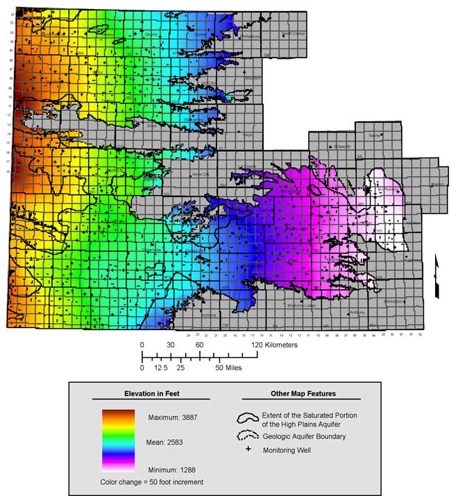
Figure 12. Kriging standard deviation for 2006 water table elevations.
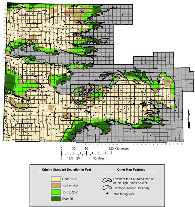
The contour levels used on the kriging error map, 13.6 feet, 15.5 feet, and 25 feet, represent the 60th, 75th, and 90th percentiles of the overall distribution of the kriging standard deviation values. The 60th percentile value of 13.6 feet has been chosen to roughly correspond with the 10-foot threshold contour on the kriging standard deviation map for 2003 (Olea and Davis, 2003). The nugget value of 133 sq. ft for the semivariogram model for 2006 water table elevations (Figure 7) results in a kriging standard deviation that exceeds 11.5 feet throughout most of the network, so that the 10-foot standard deviation threshold used to identify network holes in earlier years cannot be applied to this map. Accordingly, we will use a standard deviation of 13.6 feet in the identification of network holes (Section 9) instead. As is apparent from Figure 12, the kriging error map primarily reflects the distance to the nearest measurement point. This distance is scaled according to the semivariogram model to produce the estimated standard deviation value and changes in the nugget value will have a large impact on the prevailing value of standard deviation throughout most of the network, where separation distances are small. The configuration of the standard deviation contours, reflecting the spatial distribution of the measurement points, is more important than the contour levels themselves, which are overly sensitive to fairly small changes in the semivariogram model.
Figure 13 shows the omnidirectional semivariogram for the water-level changes over the five-year period from 2001 to 2006. The exponential semivariogram model, with a range of 74 km, nugget of 4.6 sq. ft, and sill of 40.4 sq. ft, was fitted to the empirical semivariogram using weighted nonlinear least squares (Olea, 1996). This semivariogram exhibits a shorter range and somewhat lower level of variability than that for the 2000 to 2005 declines, which had a range of 93 kilometers, nugget of 8.8 sq. ft, and sill of 44.8 sq. ft, but is very similar in character otherwise.
Figure 13. Omnidirectional semivariogram for changes in water level over the five-year period from 2001 to 2006.
Figure 14 shows the results of the kriging crossvalidation analysis for the water-level declines between 2001 and 2006. These crossvalidation results are very similar to those for the 2000 to 2005 declines reported in Bohling and Wilson (2005).
Figure 14. Kriging crossvalidation results for 5-year water-level changes.
Figure 15 is a map of the kriged water level declines between 2001 and 2006. The pattern and level of water level declines is again similar to past 5-year intervals and roughly mirrors areas with relatively higher reported ground-water use (Wilson et al., 2002). The most notable decline areas (those with multiple wells displaying the same behavior) can be seen running from Lakin and Garden City to Meade, between Hugoton to Liberal, southern Wallace County, and through the interior of Sherman, Thomas, and Sheridan counties. In contrast to past 5-year patterns, notable rises in the water table can be seen in wells along the Reno/Stafford and Harvey/Sedgwick county lines and eastern Morton County.
Figure 15. Kriged water level declines for the five-year period from 2001 to 2006.
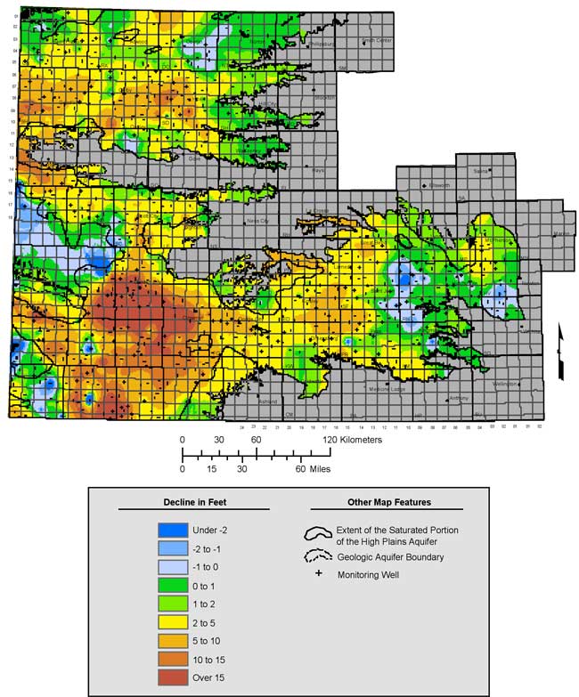
Figure 16 shows the omnidirectional semivariogram for the water-level changes from 2005 to 2006, along with the best-fit semivariogram model. The fitted model is exponential with a range of 42 km, a nugget of 1.43 sq. ft, and a sill of 6.47 sq. ft. This model is fairly different in character from that for the 2004 to 2005 declines, which was spherical with a range of 67 km, a nugget of 4.5 sq. ft, and a sill of 5.8 sq. ft (Bohling and Wilson, 2005). Although the lower nugget for the 2005 to 2006 decline semivariogram indicates smaller short-scale variability, overall the 2005 to 2006 declines seem to exhibit a higher level of spatial variability than the 2004 to 2005 declines, as indicated by the shorter range and higher sill.
Figure 16. Omnidirectional semivariogram for changes in water level between 2004 and 2005 measurement campaigns.
Figure 17. Kriging crossvalidation results for changes in water level between 2005 and 2006.
The nugget for the 2005 to 2006 decline semivariogram is approximately 22% of the sill, whereas the nugget for the 2001 to 2006 semivariogram is approximately 11% of the sill, meaning that the one-year declines exhibit considerably more short-scale variability than the five-year declines. Consequently, the crossvalidation results for the one-year declines (Figure 17) are significantly worse than those for the five-year declines (Figure 14). The smoothing effect of interpolation is readily apparent in Figure 17. Although the actual declines range from -26.8 to 23.3 feet, the estimated declines at the measurement wells range only from -10.6 to 7.3 feet. This smoothing effect must be kept in mind when considering the kriged decline map: the interpolated decline surface is almost certainly smoother than reality.
Table 5 contains the results of an analysis of variance of the kriging crossvalidation errors for the 2005 to 2006 declines against the exogenous variables describing the measurement process and well characteristics. The crossvalidation errors describe the extent to which the decline at a well is out of keeping with those at nearby wells, with a positive error indicating that the actual decline is lower than expected based on declines at nearby wells, and vice versa.
Table 5. Analysis of variance of kriging crossvalidation errors for 2005 to 2006 declines.
| Source | Df | Sum of Sq | Mean Sq | F Value | Pr > F |
|---|---|---|---|---|---|
| Measurer | 18 | 32.62 | 1.812 | 0.3996 | 0.988 |
| Downhole.Access | 1 | 1.46 | 1.465 | 0.3230 | 0.570 |
| Weighted.Tape | 1 | 0.69 | 0.693 | 0.1528 | 0.696 |
| Well.Use | 4 | 14.90 | 3.726 | 0.8216 | 0.511 |
| Oil.On.Water | 1 | 0.03 | 0.029 | 0.0064 | 0.936 |
| Chalk.Cut.Quality | 2 | 10.05 | 5.028 | 1.1088 | 0.330 |
| Aq.Group5 | 4 | 47.26 | 11.815 | 2.6056 | 0.034 |
| Residuals | 1115 | 5055.89 | 4.534 | ||
| Residual standard error: 2.13 feet | |||||
These results are dramatically different from those based on the raw decline values (Table 3), with this analysis showing no significant effect for any factor except aquifer group, which is significant at the 5% level (probability of a larger F statistic by chance is 3.4%). This ANOVA shows that none of the exogenous variables describing the measurement process has a systematic influence on the crossvalidation errors, or the degree to which a measurement is out of keeping with neighboring measurements, indicating that the measurement process appears to be highly reliable. This ANOVA almost certainly provides a more accurate assessment of the quality of the measurement program than that based on the declines themselves, since the decline residuals filter out the confounding influence of spatial trends.
Figure 18 is the kriged map of water-level declines from 2005 to 2006 which roughly follows the same pattern and relative decline levels as seen from 5-year period of 2001 to 2006. Of interest is the area between Hugoton and Liberal in eastern Stevens and western Seward counties. Between 2003 to 2004 and 2004 to 2005, this particular region showed notable rises in the water table despite widespread drought conditions. However the wells in this region show a reversal in that trend with notable declines between 2005 and 2006. Water table elevations continued to rise again in western Grant and eastern Stanton counties. Areas of south-central Kansas also experienced repeated water table rises between 2005 and 2006 although not to the same level and extent as seen from 2004 to 2005.
Figure 18. Kriged Water Level Declines for One-Year Period from 2005 to 2006.
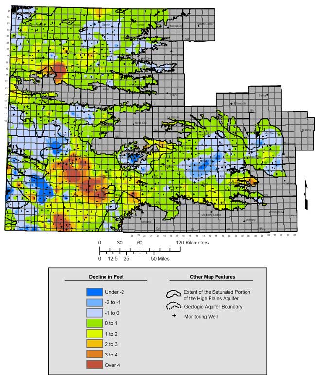
Figure 19 shows the average annual and cumulative water level declines for the High Plains aquifer region, together with the average annual growing season precipitation over the region for the decade from 1996 through 2005. The average annual declines have been computed as the average difference in depth to water measured in all network wells within the High Plains aquifer extent that were measured in both winters spanning the year in question. For example, the 1996 average decline is based on data from all the wells measured in both January 1996 and January 1997. Each annual decline is plotted as a vertical line in the middle of the appropriate year. The cumulative average annual decline, represented by the triangles plotted at successive Januaries, is simply the sum of the average annual declines since January 1996. The squares represent a different estimate of cumulative average decline, computed by comparing depth measurements in each January directly to January 1996 measurements, meaning that the average is over all wells that were measured in both 1996 and the year in question. The two estimates of cumulative decline would be the same if exactly the same wells had been measured every year. Fortunately, the results are not very sensitive to the changes in the set of measured wells over the years. The estimated growing season precipitation over the High Plains region, represented by the diamonds, is also plotted in the middle of each year. The precipitation values in Figure 19 and Table 6 are based on monthly precipitation data obtained from the National Climate Data Center (NCDC) at http://lwf.ncdc.noaa.gov/oa/ncdc.html. The monthly values were used to calculate total annual and seasonal precipitation. Seasonal precipitation is defined as the total monthly precipitation from the months of March through October. Available precipitation records run through November of 2005 which prohibits the total annual 2005 calculation.
Note that the decline axis in Figure 19 is oriented positive downward, since positive declines represent an increase in depth to water. It is clear that the annual declines reflect precipitation variations to a large degree, as would be expected.
Table 6 contains both the precipitation data and the decline data plotted in Figure 19, with the addition of the estimated annual precipitation over the year and showing only the first estimate of the cumulative decline values, that obtained by summing the average annual decline estimates.
Figure 19. Average annual and cumulative declines and growing season precipitation over High Plains aquifer region over the past decade.
Table 6. Annual and seasonal precipitation (inches), and annual average and cumulative average declines, 1996-2005.
| Year | Annual Precip (Inches) |
Seasonal Precip (Inches) |
Average Annual Decline (Feet) |
Cumulative Average Annual Decline (Feet) |
|---|---|---|---|---|
| 1996 | 26.35 | 24.31 | -0.13 | -0.13 |
| 1997 | 25.68 | 22.24 | -0.29 | -0.42 |
| 1998 | 23.02 | 19.06 | 0.37 | -0.05 |
| 1999 | 23.24 | 21.34 | 0.34 | 0.29 |
| 2000 | 22.29 | 19.91 | 1.18 | 1.47 |
| 2001 | 20.18 | 17.18 | 0.92 | 2.40 |
| 2002 | 16.73 | 15.21 | 1.98 | 4.37 |
| 2003 | 19.15 | 17.47 | 1.18 | 5.56 |
| 2004 | 24.90 | 22.21 | 0.14 | 5.70 |
| 2005 | -- | 20.54 | 0.57 | 6.27 |
The kriging error (standard deviation) map for the 2006 water-table elevations (Figure 15) indicates areas of the High Plains aquifer where suitable well control, in terms of spatial distribution, is lacking. These areas are referred to as network "holes" and are caused by a lack of depth-to-water measurements in those locations. One reason holes occur is that a monitoring well becomes unmeasurable or has been permanently removed or capped. In these cases, a new replacement well is needed. In other cases, a network hole will occur because an existing monitoring well could not be measured for that year because, for example, it was physically inaccessible or was being pumped at measurement time. In these cases, where the lack of a measurement is thought to be temporary in nature, a search is not made for a replacement well. If a measurement cannot be obtained for three years, a replacement well is identified.
Replacement wells are found by placing a hexagonal grid over the kriging error maps (Olea, 1984). Each hexagon cell is roughly 16 square miles in size and the goal is to identify a replacement well at the center of the grid. The grid center is also referred to as the hole center. Figure 20 shows the 16 network hole centers that were identified based on the 2006 measurement campaign. Only four of the network holes represent locations where existing network wells need to be replaced: two due to wells that became physically inaccessible and two due to provisional wells that have now been deemed unsuitable. Most of the other identified holes are along the fringes of the aquifer where it has been difficult to locate suitable measurement wells.
For each hole center, a list of well candidates is selected from the three major inventories of ground-water wells in Kansas. Those databases are the Water Well Completion Records (WWC5), the Water Information Storage and Retrieval Database (WIZARD), and the Water Information Management and Analysis System (WIMAS). Wells within 1 to 2 miles, and if needed, 3 miles from the hole centers are reviewed for potential inclusion in the monitoring network. The preferred type of replacement well is a well constructed for observation purposes or a newly constructed irrigation well. Once the list of well candidates has been selected, the associated landowners are contacted for permission to measure the well and include it in this voluntary program. The list of network hole centers is shown in Appendix A.
Starting in 2007, the monitoring network will be expanded to include 92 wells in northwest Kansas. These wells, referred to as "fringe" wells by DWR, have been measured each year since 2004 and will serve to cover the majority of the saturated extent of the High Plains aquifer in northwest Kansas.
Figure 20. Network holes from the 2006 measurement campaign.
The 2006 (December 2005--February 2006) water-level measurement campaign for the High Plains aquifer region shows the region experienced an average water-level decline of 0.57 feet. This is an increase in the average decline from 2004 to 2005 of 0.14 feet but is roughly half than the average annual declines observed since 2000. The spatial variations in water-level declines and their severity are tied in large part to the amount and timing of precipitation events. Precipitation affects both the potential for ground-water recharge and the need for supplemental irrigation pumping.
The trends in water-table elevations generally mirror past conditions, both in terms of spatial patterns and relative changes. A notable exception to this occurred in the area between Hugoton and Liberal in eastern Stevens and western Seward counties.
Starting in 2007, the water-level network will be expanded by 92 wells located in northwest Kansas. This addition will effectively provide depth to water measurements over the majority of the saturated extent of the High Plains aquifer in Kansas.
In a significant change of procedures compared to previous years, we have included all wells, not just those measured by KGS personnel, in the statistical quality control analysis of the 2006 measurements. This analysis showed a strong apparent dependence of the one-year water level declines on the staff member responsible for measurement. However, this effect is almost certainly due to the spatial variation in the decline values acting through the surrogate variable "measurer". The analyses of variance based on kriging crossvalidation errors at each well for both the water table elevations and one-year declines show no significant effect due to measurer. The crossvalidation errors, which indicate the degree to which a measurement differs from the neighborhood average, are probably a better indicator of measurement quality than the decline values themselves and also factor out the confounding influence of spatial trends on the analysis of variance.
The water levels for wells that have shown kriging crossvalidation errors greater than 100 feet for the past two years (Figure 9, page 20, and discussion on page 21) should be carefully examined to determine whether those wells should be retained in the network. The water table elevations for these wells seem to be systematically out of keeping with those in neighboring wells, perhaps due to the presence of significant vertical gradients between the intervals tapped by these wells and by the nearby wells. In particular, it seems quite likely that the large "errors" for wells tapping Cretaceous bedrock simply reflect significant piezometric differences between the Cretaceous aquifer system and the overlying aquifers in the vicinity of these wells.
Bohling, G. C., and B. B. Wilson, 2004, Statistical and geostatistical analysis of the Kansas High Plains water table elevations, 2004 measurement campaign: Kansas Geological Survey, Open-file Report 2004-57. [Available online]
Bohling, G. C., and B. B. Wilson, 2005, Statistical and geostatistical analysis of the Kansas High Plains water table elevations, 2005 measurement campaign: Kansas Geological Survey, Open-file Report 2005-6. [Available online]
Goovaerts, P., 1997, Geostatistics for Natural Resources Evaluation: Oxford University Press, New York, 483 pp.
Isaaks, E.H., and R.M. Srivastava, 1989, Applied Geostatistics: Oxford University Press, New York, 561 pp.
Olea, R. A., and J. C. Davis, 2003, Geostatistical analysis and mapping of water-table elevations in the High Plains aquifer of Kansas after the 2003 monitoring season: Kansas Geological Survey, Open-file Report 2003-13, 22 p, 11 plates. [Available online]
Olea, R. A., 1984, Sampling design optimization for spatial functions: Mathematical Geology, vol. 16, no. 4, p. 369-392.
Olea, R. A., 1996, XVAN: A computer program for the analysis of spatial estimation errors: Computers & Geosciences, v. 22, no. 4, p. 445-448.
Wilson, B.B., D.P. Young, D.P., and R.W. Buddemeier, 2002, Exploring relationships between water table elevations, reported water use, and aquifer lifetime as parameters for consideration in aquifer subunit delineations: Kansas Geological Survey, Open-file Report 2002-25D. [Available online]
| County | Agency | Hole Number |
UTM X | UTM Y |
|---|---|---|---|---|
| Finney | DWR | 16 | 342137.82285 | 4180568.13759 |
| Ford | KGS | 11 | 424248.58177 | 4180645.19747 |
| Greeley | KGS | 10 | 249858.55627 | 4278994.57190 |
| Kearny | DWR | 2 | 300751.48954 | 4183719.05833 |
| McPherson | DWR | 13 | 621728.56771 | 4231946.59295 |
| Morton | KGS | 1 | 256836.89436 | 4116011.22906 |
| Pawnee | DWR | 12 | 472859.04147 | 4224220.99695 |
| Sedgwick | DWR | 14 | 639610.27215 | 4182554.88957 |
| Sherman | KGS | 7 | 237705.94135 | 4361545.54956 |
| Sherman | KGS | 8 | 237619.14016 | 4346788.80004 |
| Stevens | KGS | 15 | 281542.15759 | 4098354.62996 |
| Thomas | KGS | 6 | 306249.41261 | 4347053.33888 |
| Wallace | KGS | 4 | 245886.74730 | 4303298.99052 |
| Wallace | KGS | 5 | 240961.51686 | 4295567.53126 |
| Wallace | KGS | 9 | 242046.16568 | 4310938.58997 |
| Wichita | KGS | 3 | 300751.48954 | 4282051.79274 |
WL06StatReportFinal.pdf (3.1 MB)
To read this file, you will need the Acrobat PDF Reader, available free from Adobe.
Kansas Geological Survey, Geohydrology
Placed online Aug. 7, 2006
Comments to webadmin@kgs.ku.edu
The URL for this page is http://www.kgs.ku.edu/Hydro/Levels/2006/OFR06_20/index.html