
|
|
Department of Geosciences
Fort Hays State University
600 Park Street
Hays, KS 67601
KGS Open-file Report 2004-35
Global Positioning System (GPS) data and a Geographic Information System (GIS) technique were used to calculate the volume remaining in the City of Hays, Kansas, industrial landfill. This volume was subsequently used to calculate the life expectancy of the landfill. Constraints on the calculation included annual "waste" disposal, annual "cover application," and "final cover" application. The calculated life expectancy was determined to be 32-36 years depending on the annual "range" of waste brought to the landfill.
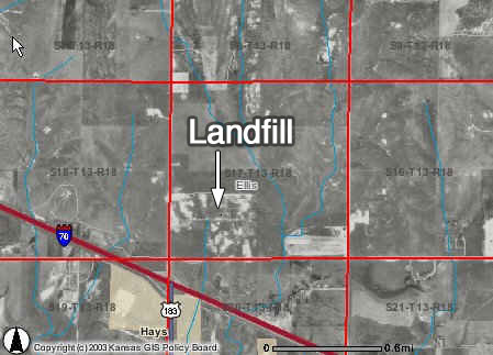
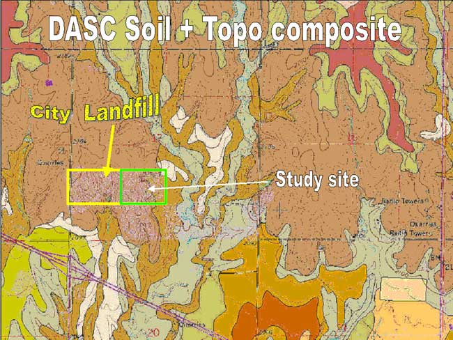
The Kansas Department of Health and Environment (KDHE), Bureau of Waste Management (BWM), reviews the "Operating Plan" of all Kansas municipalities and requires each of them to submit a detailed plan regarding their landfill (figure 1; SW sec. 17; T. 13 S.; R. 18 W.). The review consists of 18 items covering composition of waste; expected volume of waste; waste-screening procedures; disposal, placing, compacting, and covering of waste; safety procedures; cover-application rate; storm-water control; equipment used; contingency-emergency plans; final or temporary closure; drawings illustrating phases and development stages; proposed capacity and expected life; quality assurance; communication; record keeping; access control; and dust control.
Figure 1--KanView images of the Landfill [also see DASC Soil + Topo images at end of report].
After coming to an agreement with the City of Hays and receiving a grant from the Kansas Geological Survey, three faculty and five undergraduate students (the 'team') from Fort Hays State University (FHSU) embarked on the task of calculating the volumetric and life expectancy items of the operating plan in December of 2003.
The team met with John Braun (Assistant Public Works Director) and Karen Randa (Inspector), City of Hays Public Works Department, several times at the landfill site to reconnoiter the site, discuss the city's needs, and plan a field procedure to gather data. The City provided FHSU with both hard copies and digital format (on CD) of a digital orthophoto quad of the site, GPS data collected by the City in the summer of 2003, and two AutoCAD data files and maps that covered GPS points and surface contours of the present state of the landfill.
The City data were in State Plane coordinates (in feet) and the team preferred to work with UTM coordinates (metric). After making several conversions of the City data and creating several 2D and 3D images in ArcGIS and Spatial Analyst, we decided that we needing a higher resolution of GPS data points focused on the main proposed fill area of the landfill. We felt that the City data were insufficient to generate adequate interpolation points, and we also encountered problems with merging data files with ArcGIS (figs. 2 and 3). Their data covered more than the area targeted for this project. We subsequently conducted a new GPS survey on February 13, 2004.
Figure 2--City GPS data, surface displayed using interpolated model.
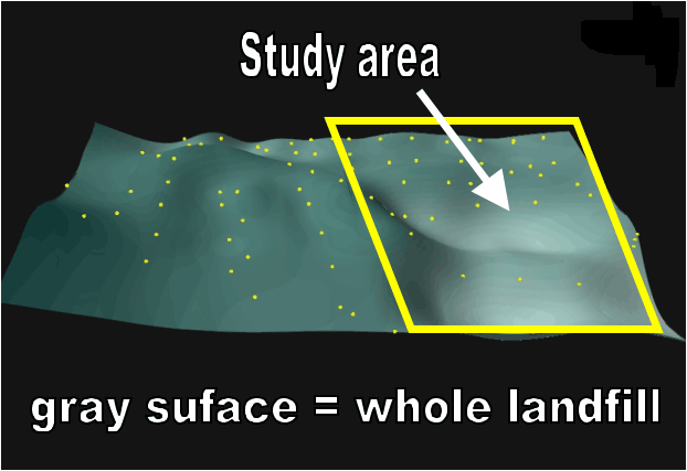
Figure 3--City GPS data, surface displayed using triangulated irregular network (TIN).
A Leica GS-50 GPS unit was used to collect 142 geospatially referenced points over a grid marked with flags within the targeted fill area. The perimeter of this area was determined using the pre-established AutoCAD contour map provided by the City. The new GPS points were concentrated in areas of greatest topographic relief in order to increase resolution control. Points were recorded in UTM coordinates, WGS-84. Samples of landfill material and onsite digital photos were also taken of the area and GPS surveying (figs. 4-6).
Figure 4--Entrance to City of Hays landfill.
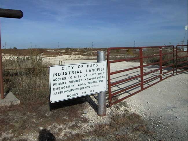
Figure 5--Team collecting samples from landfill.
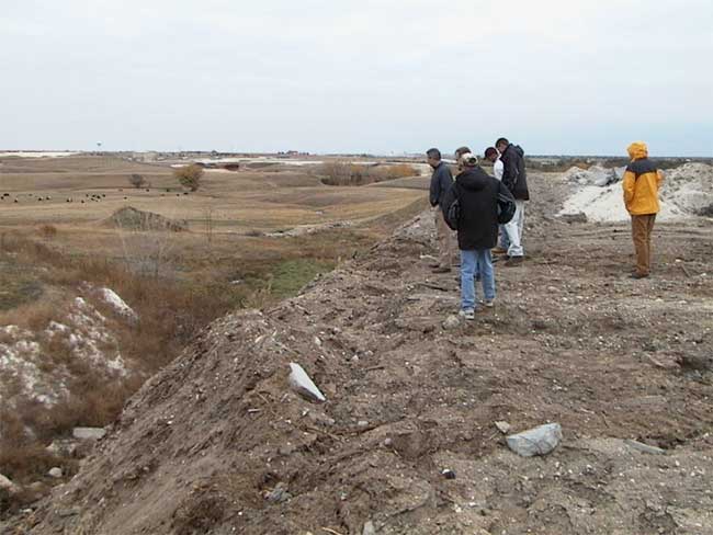
Figure 6--Photographing and sampling landfill.
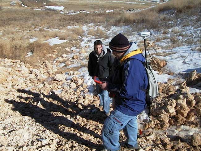
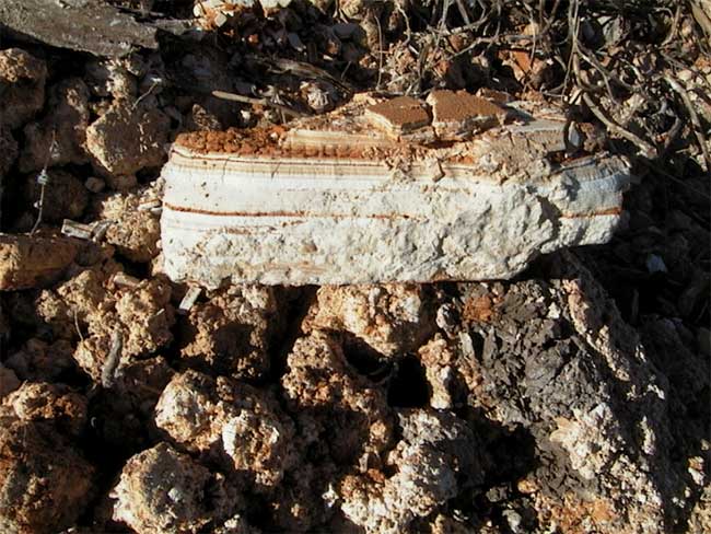
Figure 7--Sample from City of Hays landfill.
GPS point sets were downloaded as ESRI shapefiles using Leica DATAPRO software and interpolation surfaces were checked against the actual surface using onsite photos and DOQQ provided by DASC. New contoured images produced in ArcGIS Spatial Analyst were more accurate due to the greater number and more even spacing of the GPS points. However, a few areas were targeted where we desired further resolution. We thus gathered an additional 40 GPS data points on February 19, 2004, for a total of 182 GPS points. Karen Randa was present for this final GPS shoot (fig. 5).
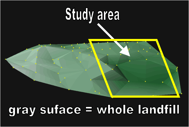
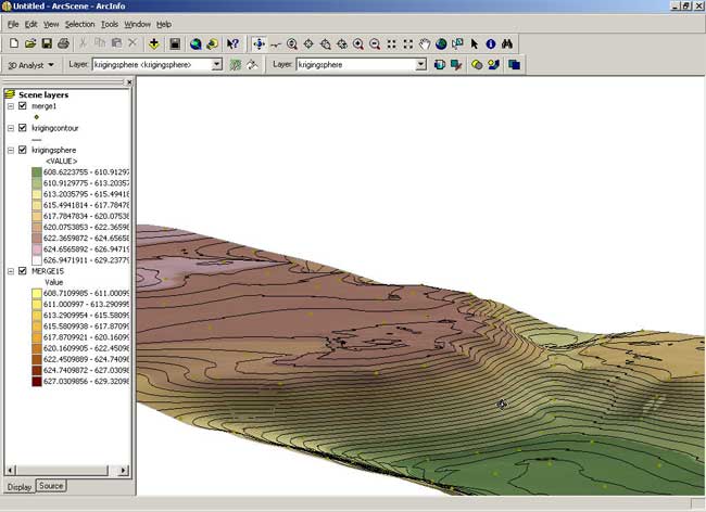
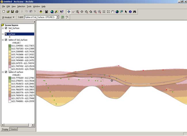
The team began the GIS lab volumetric analysis on February 20, 2004. Perimeter and interior point sets were merged for a more accurate coverage. A series of interpolation surfaces were then created using ESRI's Spatial Analyst software package; these surfaces were then compared to the aerial photos and site photos of the site, in order to determine which interpolation algorithm best replicated the actual existing surface. Surfaces were created using the Inverse Distance Weighted method, the Regularized Spline method, the Tension Spline method, and Kriging (fig. 8). After extensive examination, the team decided that the surface created by the Tension Spline method best conformed to the contours of the actual surface, so Tension Spline surfaces were used in all further analysis.
Figure 8a--Surface created by ESRI's Spatial Analyst--Tension Spline method. A larger version of this figure is available.
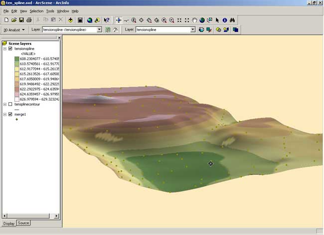
Figure 8b--Surface created by ESRI's Spatial Analyst--Inverse Distance Weighted method. A larger version of this figure is available.
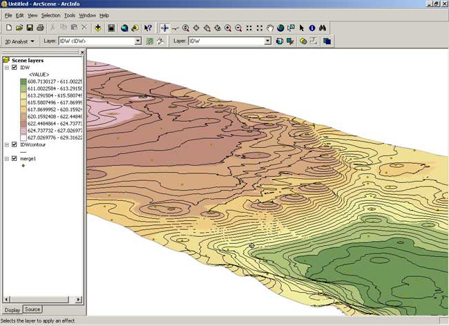
Figure 8c--Surface created by ESRI's Spatial Analyst--Kriging method. A larger version of this figure is available.
In order to obtain the eventual volumetric calculation in the proper units, the surface projection was converted from a geographic projection, using decimal degrees as units of measure, to UTM coordinates (zone 14N), using meters. Once this was done, a three-dimensional surface was generated in ArcScene (3D view) to give "real world" visuals of the landfill.
KDHE standards required that the final configuration of the filled landfill possess a slope of no steeper than a 3:1 rise/run ratio (figs. 9 and 10). All calculations concerning the useful life of the landfill necessarily had to take this standard into account. It was decided that the best approach was to generate a hypothetical 3:1 slope surface using precalculated elevation points, representing the final filled surface of the landfill, rasterize this surface, and perform a cut and fill calculation using this hypothetical filled surface and the tension spline surface generated using the GPS points, in order to obtain a volumetric calculation.
Figure 9--Team working on calculations for slope of landfill.
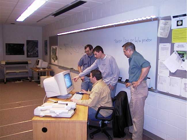
Figure 10--Landfill-slope calculations.
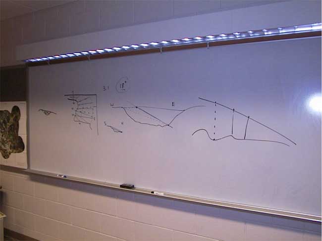
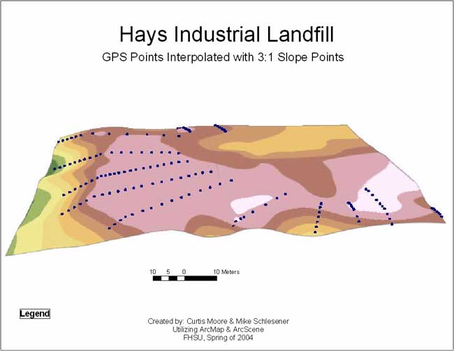
A long discussion about possible ways to calculate a hypothetical surface with a 3:1 slope ensued. It was finally decided to manually calculate the slope from elevation points assigned along 12 transects running from the highest escarpment elevation to the edge of the landfill area. Elevation profiles were created in 3D Analyst for all 12 transects, and hypothetical elevation points were assigned at 3.0 meter intervals along each transect (figs. 11 and 12).
Figure 11--Elevation profile of 3:1 slope model. A larger version of this figure is available.
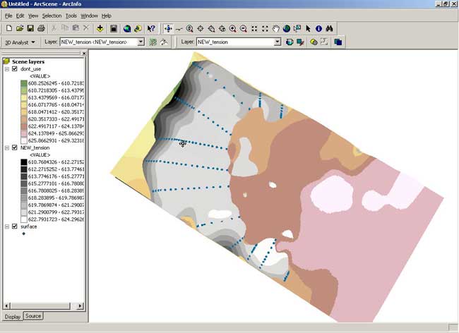
Figure 12--3D model of 3:1 slope for landfill. A larger version of this figure is available.
Because the rise/run was equal to .3333, the maximum distance from the highest elevation to the bottom of the slope was calculated by dividing the maximum height of the slope by 0.3333. Hypothetical elevation points for the slope were calculated by multiplying distance by 0.3333 and then adding the original base elevation of each point. ArcCatalog was then used to manually input the hypothetical elevation points and to create a shapefile of the hypothetical "filled" surface. This surface was then rasterized, and a cut/fill analysis was performed, using the ESRI Spatial Analyst "Cut/Fill" function. Output cell size was set to 1 meter, in order to obtain a usable volumetric calculation (figs. 13 and 14). Six profiles of the three layers used to calculate the final volumetrics are found in Appendix A.
Figure 13--3D model of volumetric calculation for landfill. A larger version of this figure is available.
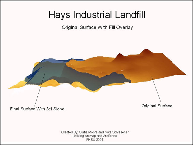
Figure 14--Volumetric calculation model for hypothetical "filled" landfill. A larger version of this figure is available.
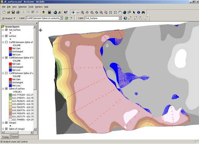
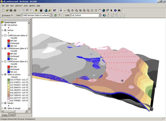
The Cut/Fill calculation was performed as outlined above. Using Cut/Fill, the total potential volume of the landfill was calculated to be = 78,543 m3 (figs. 15 and 16). In order to ensure accuracy, the team double-checked the methodology of the procedure with ESRI (Environmental Systems Research Institute) Technical Support Staff and also double-checked the method against similar published volumetric work. Using these resources as checks, the method used, and hence the final volume calculation, were determined to be sound.
Figure 15--3D model of potential "filled" landfill. A larger version of this figure is available.
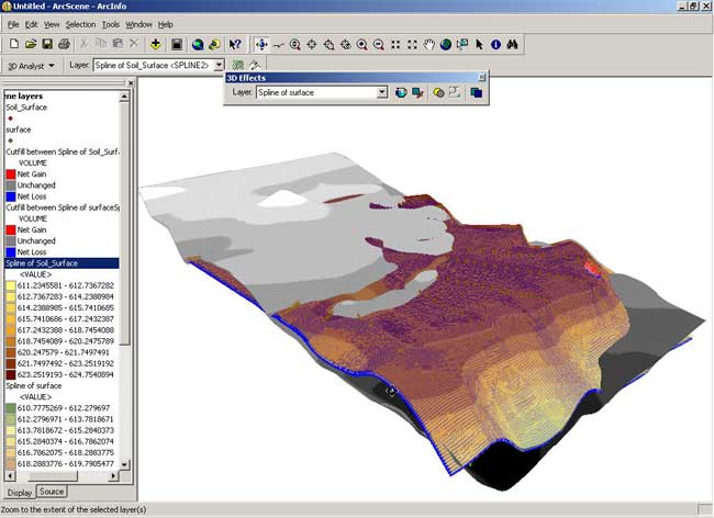
Figure 16--Potential volume landfill model. A larger version of this figure is available.
With the total potential volume of the landfill calculated, it became possible to estimate the usable "lifespan" of the landfill, once information about future dumping became available. The City provided this information, in the form of the densities of material involved in dumping and the estimated number of loads to be dumped per year. The team calculated the volume of this material, and these values were converted to ft3 and m3. The resulting estimated volume was divided into the total potential volume calculated for the landfill in order to determine the life expectancy of the landfill based on current usage.
In order to meet required KDHE standards, a yearly "cover" fill was required; according to information provided by the City of Hays, this cover would add an extra 2-4 inches of overburden per year. This figure was averaged to 3 inches per year, with a total final cover of 1.5 feet, also required under KDHE standards. This was estimated to take up roughly 40% of total fill volume, reducing total calculated fill volume from 78,543 m3 to 47,539 m3 (figs. 17 and 18).
Figure 17--Reconfigured model of "filled" landfill taking cover into consideration. A larger version of this figure is available.
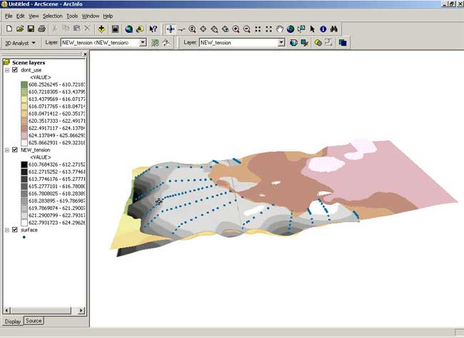
Figure 18--Model of reconfigured fill volume using "cover" fill requirement. A larger version of this figure is available.
Based on the data provided us by the City of Hays, our GPS data, and GIS-derived volumetric data, we conclude that the life expectancy of the City of Hays' Industrial Landfill ranges from 32 to 36 years. The results of our calculations are outlined below.
Volumetric Calculations:
Estimated Life of Landfill Calulations
Total Volume of Trash and Soil Cover Per Year
Total Volume Divided by Annual Volume Estimates
ArcGIS, v. 8.3, ESRI
ArcGIS Spatial Analyst, v. 8.3, ESRI
Data Pro, Leica
GIS data files and instructions: 1.5 MB Zip archive of folder
Profiles:
Soil and topographic data layers in landfill area.
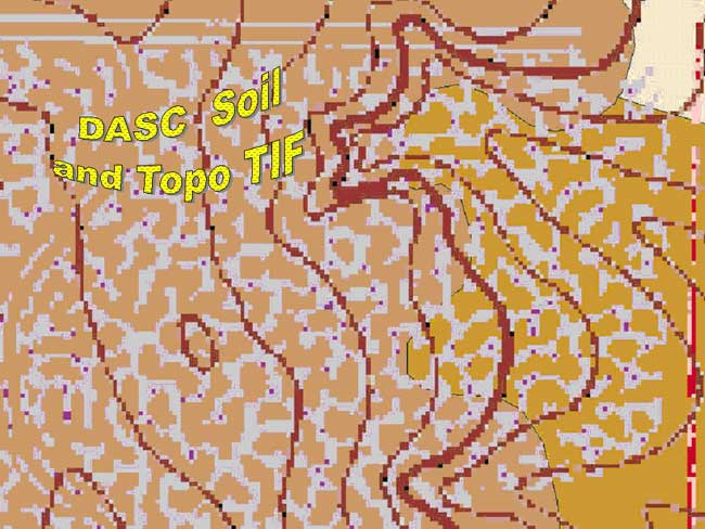
Soil and topographic data layers in study area.
Kansas Geological Survey, Hays Landfill
Comments to webadmin@kgs.ku.edu
Web version July 2004.
URL=http://www.kgs.ku.edu/Publications/OFR/2004/Hays/index.html