Kansas Geological Survey, Bulletin 233, p. 33-42
by
G. Nicolis1 and C. Nicolis2
1Université Libre de Bruxelles
2Institut Royal Météorologique de Belgique
Geophysical phenomena are often characterized by complex, random-looking deviations of the relevant variables from their average values. Typical examples of such aperiodicity are the intermittent succession of Quaternary glaciations as revealed by the oxygen isotope record of deep-sea cores of the last 106 years or the pronounced spatial disorder characterizing geologic materials. A major task of the geoscientist is to reconstitute from this type of record the principal mechanisms responsible for the observed behavior. Traditional approaches attribute the complexity encountered in the record of a natural variable to external uncontrollable factors and to poorly known parameters whose presence tends to blur fundamental underlying regularities. Here, we consider that complexity might be an intrinsic property generated by the nonlinear character of the system's dynamics. We review bifurcations, chaos, and fractals, three important mechanisms leading to complex behavior in nonlinear dynamic systems, and stress the role of the theory of nonlinear dynamic systems as a major tool of interdisciplinary research in the geosciences. The general ideas are illustrated on the dynamics of Quaternary glaciations and the dynamics of tracer transport in a sediment.
An Acrobat PDF file containing the complete paper is available (788 kB).
Much of our understanding of the earth's past environmental and climatic conditions rests on the ability to decipher geologic data. This involves in turn a number of highly nontrivial intermediate steps. To begin with, the time sequence of events must be reconstructed from the spatial distribution of, say, a representative tracer within a sediment, or, put differently, the space axis along the geologic material has to be converted into a time axis along which past history begins to unfold. Furthermore, a typical time series obtained in this manner displays considerable complexity reflected by the lack of any obvious periodicity and by the occurrence of random-looking excursions of the relevant variables from their average levels. Two questions of obvious concern are therefore how to decipher the message of such a time series and how to determine the roles that systematic effects and randomness play.
When confronted with a complicated or even at first sight erratic succession of events, the first explanation that comes to mind is that the phenomenon of interest is blurred by the presence of a great number of parasitic variables and poorly known parameters that hide some fundamentally simple underlying regularities. Traditional statistical methods provide useful algorithms for extracting the relevant signal from what is believed to be random background noise. Our principal aim here is to draw attention to the fact that in addition to such considerations it is important to adopt complementary approaches based on a more dynamic view of the underlying phenomena (Nicolis and Nicolis, 1987).
The need for a dynamic approach stems from recent developments in the physical and mathematical sciences that indicate that the stable and reproducible motions which dominated science for centuries no longer symbolize our physical world (Nicolis and Prigogine, 1989). Experiments on quite ordinary physicochemical systems on the laboratory scale and the study of mathematical models reveal the existence of instabilities that amplify small effects and drive the systems to alternative states. These nonlinear phenomena are sources of intrinsically generated complexity and unpredictability. Furthermore, some of the states arising through this mechanism present the characteristics of deterministic chaos: Despite their generation by a well-defined set of laws, they give rise to aperiodic, random-looking behavior. Finally, coming back to geology, geologic materials are complex media characterized by a pronounced disorder entailing that a phenomenon embedded in such a material becomes a complex process whose instantaneous rate is likely to vary continuously, depending on the locally prevailing conditions. Clearly, in light of these observations, in large classes of natural phenomena it may be meaningless to eliminate the variability and to keep only the mean as the most representative part of the behavior.
In the next section we summarize the principal mechanisms leading to complex behavior in nonlinear dynamic systems. As an illustration of these ideas, we first consider the dynamics of Quaternary glaciation in connection with the oxygen isotope record of deep-sea cores. Then we analyze from a similar point of view the role of the complexity of the geologic material in the dynamics of tracer transport in a sediment. Finally, we close with comments on the potential interest of the approach developed in this article.
The evolution of a natural system over the course of time is conditioned by two major factors: (1) a set of laws governing the individual elements constituting the system and their interactions and (2) a set of constraints acting from the external world that are usually manifested by means of control parameters. Typical examples are temperature gradient, stress, or the structural characteristics of the underlying material, affecting, in turn, such properties as transport coefficients or chemical rate constants.
Let Xi, i = 1, …, n, be the relevant variables. We write the rate of change in time in the form
dXi / dt = vi (X1, …, Xn; λ, μ, …), i = 1, …, n (1)
where vi are the evolution laws and λ, μ, … are the control parameters. An illustration of Eqs. (1) in the field of geology is provided by the reaction-transport equations governing the dynamics of a set of tracers in a sediment. Closer to our preoccupations here, we can consider Eqs. (1) to represent processes related to global environmental change, such as coupled energy and mass transfer between the hydrosphere, cryosphere, and atmosphere, which leaves a permanent record on geologic material through a passive quantity acting as an indicator. A typical example of this interpretation is provided by the δ18O isotope record in connection with Quaternary glaciations.
Whatever the detailed interpretation of Eqs. (1) might be, a common feature shared by large classes of systems is that the vi are nonlinear functions of the state variables. This ubiquity of nonlinearity in nature stems primarily from the numerous feedbacks exerted between the different components of the system (e.g., surface-albedo feedback). Additional sources of nonlinearity can arise from the non-Newtonian character of a material (state-dependent transport coefficients) or from hydrodynamic flow.
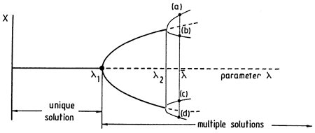
Nonlinearity is a source of intrinsically generated complex behavior and unpredictability, in the sense that more than one outcome of the evolution is possible (Guckenheimer and Holmes, 1983; Nicolis and Prigogine, 1989). Figure 1 depicts a typical scenario of the way the solutions X of a nonlinear dynamic system behave when a parameter λ built into the system is varied. At the values λ1, λ2, λ3, … of the parameter, usually referred to as bifurcation points, new branches of solution are generated. In general, these bifurcation cascades produce several simultaneously available states, which we refer to as attractors (branches a to d for the value λ = ![]() in fig. 1). Which of these states will actually be chosen depends on the initial conditions. This property confers to the system a high sensitivity and a markedly random character, because the initial conditions are history dependent and can be modified by fluctuations or by external perturbations. Therefore the dynamics of a multistable system actually is an aperiodic succession of intermittent jumps between coexisting attractors. This view, which will be taken up in more detail in the next section, is reminiscent of a great number of natural processes involving abrupt transitions.
in fig. 1). Which of these states will actually be chosen depends on the initial conditions. This property confers to the system a high sensitivity and a markedly random character, because the initial conditions are history dependent and can be modified by fluctuations or by external perturbations. Therefore the dynamics of a multistable system actually is an aperiodic succession of intermittent jumps between coexisting attractors. This view, which will be taken up in more detail in the next section, is reminiscent of a great number of natural processes involving abrupt transitions.
Figure 1--Typical bifurcation diagram of a nonlinear dynamic system.
A convenient representation of the states that can be reached by a system beyond a bifurcation is provided by the phase space, the space spanned by the full set of variables X1, …, Xn participating in the dynamics (Nicolis and Prigogine, 1989; Guckenheimer and Holmes, 1983). The nature of the phase space portrait depends on whether the system is conservative or dissipative. Experiment shows that most systems encountered in nature are dissipative, a property that shows up through an irreversible evolution to a preferred set in phase space, which we call an attractor. Attractors enjoy the important property of asymptotic stability, that is, the ability to damp perturbations. This in turn ensures a certain degree of reproducibility of the behavior.
Whatever its detailed nature, an attractor has a measure in phase space that is equal to 0. In other words, in a phase space of n dimensions the dimensionality d of the attractor will satisfy the strict inequality d < n. Actually, in many cases d is much less than n, indicating that a drastic reduction of the description of the system is possible. The simplest attractors are zero-dimensional (point) and one-dimensional (limit-cycle) manifolds, as depicted in fig. 2. However, in many instances bifurcation cascades lead the system to the regime of deterministic chaos (Baker and Gollub, 1990; Bergé et al., 1986). Figure 3 depicts a typical attractor describing chaotic dynamics obtained by numerical integration of a three-variable model system (Rössler, 1979):
dx / dt = -y - z,
dy / dt = x + ay,
dz / dt = bx - cz + xz. (2)
Figure 2--Evolution toward a point attractor (a) or limit cycle attractor (b) in a dissipative dynamic system.
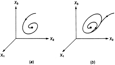
Figure 3--Chaotic attractor obtained from numerical integration of the system of Eqs. (2). Parameter values: a = 0.38, b = 0.3, c = 4.5.
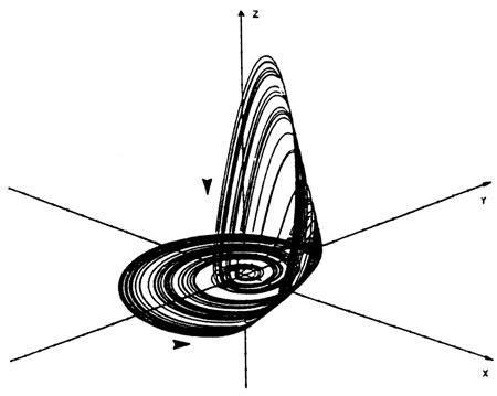
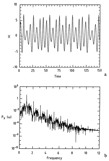
Figure 4 illustrates two ubiquitous features shared by all chaotic attractors. First, contrary to what happens in a periodic limit-cycle attractor (fig. 2b), the trajectory never closes back onto itself (fig. 4a); second, in addition to certain well-defined characteristic frequencies, a chaotic attractor generates a broadband spectrum reminiscent of random noise (fig. 4b). Chaotic attractors thus show that irregular, aperiodic behavior sharing some features of a random process can be generated by a dynamic system governed by perfectly deterministic laws of evolution.
Figure 4--(a) Typical aperiodic time evolution of a variable in the regime of deterministic chaos. (b) Power spectrum associated with this variable, displaying the broadband character usually attributed to random noise.
Let us have a closer look at the structure of the attractor (fig. 3). We observe two opposing trends: an instability of motion tending to remove the phase space trajectory away from the reference state x = y = z = 0 (horizontal arrow) and the bending of the outgoing trajectories followed by their reinjection into the vicinity of this state (vertical arrow).
The unstable motion on the attractor (as opposed to the stability in the directions transverse to the attractor) is reflected in the sensitivity of the trajectories on the attractor to minute changes in the initial conditions, as a result of which two initially nearby states diverge, on average, in an exponential fashion. The characteristic rate of divergence σL is referred to as the (largest) positive Lyapounov exponent of the system. For the model of Eqs. (2) it turns out that (σL = 0.15 bit per unit of time.
What makes the geometric object in fig. 3, which is generated by a one-dimensional curve, the phase space trajectory, capable of accommodating all this complexity? A detailed study shows that during the different reinjection cycles the attractor undergoes successive foldings. Stated differently, a section of the attractor transverse to these folded sheets looks like a line from which an increasing number of segments of decreasing size are removed (fig. 5). Present-day mathematics provides us with models of this kind of object, which is referred to as a fractal; the particular fractal in fig. 5 is known as a Cantor set (Mandelbrot, 1977). A key mathematical concept characterizing fractal objects is the correlation dimension v, expressing essentially the way the number of points N, on the attractor at a distance r from a given point varies on average with r as r goes to 0 (Grassberger and Procaccia, 1983; Bergé et al., 1986; Baker and Gollub, 1990):
Nε = rv. (3)
Fractals can be distinguished from traditional objects described by Euclidean geometry because v is strictly larger than the Euclidean dimension. For instance, in the limit of an infinite number of foldings, a Cantor set (fig. 5) is composed of an infinity of disconnected points and thus has a Euclidean dimension equal to 0. Yet its fractal dimension turns out to be between 0 and 1. This entails that in the full phase space the attractor of fig. 3 is a fractal object of dimension between 2 and 3.
Figure 5--Successive steps leading to the Cantor set.
A number of alternative definitions of dimension of fractal objects have been proposed to be able to distinguish between uniform attractors, in which all regions are visited with practically the same probability, and highly nonuniform attractors. In general, all these dimensions and the Lyapounov exponents (σL cannot be computed analytically. Algorithms are currently available that allow the determination of v and σL from the knowledge of a time series pertaining to the evolution of a single variable. We sketch this procedure in the next section in connection with paleoclimatic data. We close the present discussion by pointing out that the coexistence of the two antagonistic trends of overall stability and reproducibility of the attractor on the one side and of instability of motion on the attractor itself on the other side makes deterministic chaos the natural model for understanding objects whose complexity stems from the coexistence of randomness and order. As pointed out in the introduction, such objects should be important in the geosciences. The situation is different in the presence of random noise, because in this case there is no mechanism capable of keeping the system confined to a privileged part of its state space.
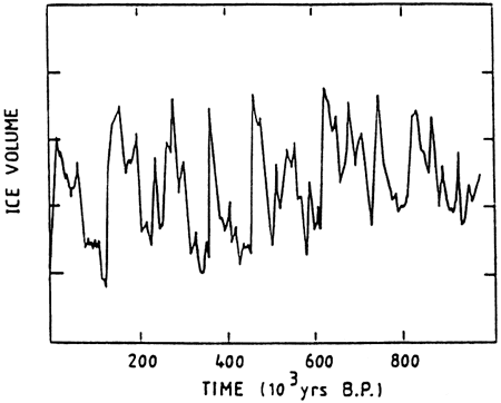
The quantitative study of a natural system is based on the measurement of a set of relevant variables during a sufficiently long period of time. An important example of such a time series is given in fig. 6, in which the oxygen isotope record of a deep-sea core during the past 106 years is depicted (Shackleton and Opdyke, 1973). Such records are thought to provide a reliable estimate of the global ice volume present on Earth against time. We observe a number of excursions associated with the glaciation periods, the most dramatic climatic episodes of the Quaternary era. Both the position and strength of these excursions are rather irregular, although on average a time scale of 105 years is clearly emerging. In this section we comment on the origin of this variability in the light of the ideas developed in the previous section.
Figure 6--Global ice volume on earth inferred from oxygen isotope record of core V28238 (Shackleton and Opdyke, 1973).
The traditional approach in modeling complex dynamics is to consider a linear equation for the relevant variable (here the global temperature or the ice volume) subjected to random forcing. This type of approach is inadequate for the data depicted in fig. 6. Indeed, the strength of the noise needed to reproduce the large-scale glacial-interglacial excursions would be exceedingly large.
A second approach consists in introducing in the model a periodic component that takes into account the variation of the eccentricity of the earth's orbit, whose amplitude and periodicity are of the order of 10-3 and 100,000 years, respectively (Berger, 1981). It can be verified, however, that the response of such a system is of the order of the amplitude of the forcing itself, that is, much smaller than the observed response. It seems, therefore, that simple linear response-type models cannot provide us with a plausible mechanism for the Quaternary glaciations. In the language of the previous section, this means that the situation in which only one point attractor is available is not representative of the glaciation cycles. We are therefore forced to look for an alternative scenario.
A second typical possibility is that a dynamic system displaying the behavior depicted in fig. 6 possesses two coexisting attractors and performs intermittent jumps between them (Nicolis and Nicolis, 1981). This automatically implies that nonlinear effects are essential in the sense that the dynamics can no longer be expanded around a well-defined reference state and subsequently linearized to a good approximation.
A simple model corresponding to such a scenario is the globally averaged (also referred to as zero-dimensional) energy balance model for Earth:
dT/dt = v(T, λ) = 1/C [(incoming solar energy) - (outgoing infrared energy)] = 1/C (Q[1 - α(T)] - εBσT4), (4)
where T is the space-averaged surface temperature, C is the heat capacity, Q is the solar constant, α is the albedo, σ is the Stefan constant, and εB is the emissivity factor representing the deviation from blackbody radiation. The surface-albedo feedback can be readily incorporated into this picture by modeling the albedo as a stepwise linear function. The resulting energy balance is represented in fig. 7.
Figure 7--Incoming and outgoing radiative energy curves as functions of T (global average temperature). Their intersections Ta, Tb, and T0 are the steady states predicted by Eq. (4).
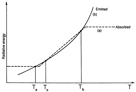
For plausible parameter values Eq. (4) can give rise to two stable steady states, Ta and Tb, representing a glacial and a more favorable climate, respectively, separated by an intermediate unstable climate, T0. If (as suggested by the record) the difference Ta - Tb is small, the system can be assumed to operate near a bifurcation point.
Climatic change necessitates a transition between states a and b. In the model elaborated so far no mechanism allowing for such a transition is present except for the trivial one, whereby the system initially at Tb (say) is perturbed and brought close to Ta. Such massive perturbations are hard to imagine. Therefore we enlarge our description by incorporating the effect of random fluctuations F(t), which are always present in a complex physical system because of the imbalances that inevitably exist between transport and radiative mechanisms. We model these fluctuations as Gaussian white noise:
<F(t)> = 0,
<F(t)F(t')> = q2δ(t - t'), (5)
where q2 is the variance of fluctuations. We write the augmented energy balance equation as
dT / dt = v(T, λ) + g(T)F(t), (6)
where g(T) represents the coupling of the internal dynamics to F(t).
This stochastic differential equation (also referred to in the literature as the Langevin equation) can be studied by the methods of the theory of stochastic processes. The principal features of the evolution predicted can be summarized as follows. Suppose that the system is started on one of its stable attractors. If the strength of the stochastic forcing F(t) is small, during a long period of time the system will perform a small-scale jittery motion around a level corresponding to this attractor. But sooner or later there is bound to be a fluctuation capable of overcoming the barrier separating this state from the other ones available, in which case over a short time interval the system will find itself on another attractor. Subsequently, it will again undergo small-scale motion around this new level until a new fluctuation drives it back to the previous state (or to a third one, if available), and so forth. This intermittent evolution looks like the record in fig. 6. Generally, it provides us with an archetype for understanding a large class of abrupt transition phenomena beyond our specific problem, for example, recurrent precipitation regimes in some areas or river or lake levels (Demarée and Nicolis, 1990).
A more quantitative study shows that the transition between attractors occurs on a time scale given by Gardiner (1983) and Nicolis and Nicolis (1981):
τa,b ≈ exp {(2/q2)ΔUa,b} (7)
The quantity ΔUa, or ΔUb is known as a potential barrier. It is defined by
ΔUa,b = U0 - Ua,b (8a)
where U0, Ua,b is the integral of the right-hand side of Eq. (4):
U(T,λ) = -∫Tv(x,λ)dx (8b)
evaluated on states T0, Ta, or Tb. By analogy to mechanics, U can be referred to as the kinetic potential, because its derivative δU/δT represents the force v responsible for the evolution. If, as expected, the variance of the fluctuations q2 is small and the barrier ΔU is finite, τa or τb will be much larger than the local relaxation time and could be in the range of glaciation time scales. In contrast, the local evolution in the vicinity of each attractor is given by the inverse of the first derivative of v evaluated on Ta or Tb. For an energy balance model it should be of the order of a year.
Despite the developed arguments, Eq. (6) cannot yet be considered a satisfactory model of Quaternary glaciations: The transitions between Ta and Tb occur at randomly distributed times, whereas the climatic record suggests that Quaternary glaciations have a cyclic character bearing some correlation with the mean periodicities of the earth's orbital variations. Let us therefore study the response of our multistable model to both stochastic and periodic perturbations. Taking the simplest case of a sinusoidal orbital forcing, one is led to
dT / dt = v(T, λ) + g(T)[ε sin ωt + F(t)], (9)
where ε and ω are the amplitude and the frequency of the forcing, respectively. It should be pointed out that ε is very small, of the order of a fraction of a percent.
The most striking result pertaining to Eq. (9) is undoubtedly the possibility of stochastic resonance (Nicolis, 1982; Benzi et al., 1982). When ΔUa ≈ ΔUb and the forcing period 2π/ω is of the order of the characteristic passage times τa,b, the response of the system is dramatically amplified. Specifically, the probability of crossing the barrier is substantially increased, and the passage occurs with a mean periodicity equal to the periodicity of the forcing. This allows us to understand, at least qualitatively, how, despite its weakness, periodic forcing may leave a lasting signature in the climatic record.
As we saw earlier, chaotic dynamics provides a second universal mechanism of evolution in the form of intermittent jumps between different levels. Let us explore this scenario for the paleoclimatic record of fig. 6. The question we raise is whether (1) on the sole basis of the time-series data one can identify some intrinsic properties of the dynamics of climate, independent of any modeling, and (2) whether the intermittency and the aperiodicity displayed in fig. 6 are the consequence of deterministic dynamics or of a random, impossible to control course of events.
The first step to be carried out in answering this question is to embed the dynamics of the system under study in phase space. This means, in particular, that one should go beyond the one-dimensional view afforded by a time series of a single variable X0(t). It can be shown that a phase space satisfying all requirements of dynamic systems theory is the phase space generated by X0(t) and its successive lags X0(t + τ), …, X0[t + (n - 1)τ]. It suffices to choose τ in such a way that these different functions are linearly independent.
Next, in each of the defined phase spaces (i.e., for each value of n), one tries to identify the nature of the set of data points, viewed as a geometric object in an n-dimensional space. Again, dynamic systems theory provides algorithms for accomplishing this. One particular quantity that can be identified in this way is the dimensionality v(n) of our data set [cf. Eq. (3)]. Once v(n) is determined, one can also obtain information on dynamic properties, such as the largest positive Lyapounov exponent σL(n), if any.
Finally, v and σL are plotted against n for increasing values of the embedding dimensionality. If these dependencies are saturated beyond some relatively small n, the system represented by the time series should be a deterministic dynamic system possessing an attractor. The saturation values of v and aL are the dimensionality and the largest Lyapounov exponent of the attractor. The value of n beyond which saturation is observed provides the minimum number of variables necessary to model the behavior represented by the attractor. On the other hand, if there is no saturation trend, the conclusion will be either that the system described by the time series evolved in a random way or that the dimensionality is too high to be revealed by the available data.
This procedure, applied to the climatic data in fig. 6, gives a fractal dimensionality of v ≈ 3.1, a positive Lyapounov exponent corresponding to a characteristic predictability time of approximately 30,000 years and a minimum value of n = 4 (Nicolis and Nicolis, 1984,1986). We thus conclude, on the basis of the data, that long-term climatic change can be viewed as deterministic unstable dynamics possessing a chaotic attractor. This provides us with a natural way to understand the well-known variability of the climatic system on this long scale. It also allows us to calculate quantitatively the limits beyond which predictions about the future become meaningless.
We close with the remark that, far from being contradictory, the last two scenarios of long-term climatic change present interesting complementarities. Specifically, the picture of a bistable system performing fluctuation-driven intermittent jumps between two states can be viewed as a shorthand description of a chaotic attractor, which, as stressed earlier, shares in many respects the features of a random process. In other words, the deterministic part and the random force v(T, λ) and F(t) in Eq. (6) represent, respectively, the large-scale structure of the underlying chaotic attractor and the effective noise that is intrinsically generated by the dynamics. In this perspective a more satisfactory approach would be to model F(t) as a highly correlated process rather than as a white noise process. The theory developed in this section can be amended to take this refinement into account without any substantial change in the overall philosophy underlying the dynamic systems approach to global environmental change.
We now turn to the mechanisms presiding in the conversion of a temporal signal witnessing a certain environmental change into a space record imprinted on a geologic material. We consider a tracer moving in a medium that, depending on the circumstances, may be a chemical substance dissolved in water, a macroscopic particle (e.g., debris of a certain biologic species) containing a radioactive isotope, etc.
As stressed already, geologic media are complex materials. They present a pronounced irregularity and fragmentation, which can hardly be viewed as a small, quantitative modification of some regular reference lattice. To capture the essence of this irregularity, we assimilate the material to a fractal (Wong, 1988). The specific choice of fractal is a major question whose answer depends on the nature of the material in a given problem. Here, we consider as a case study the abstract but typical model in which the medium can be regarded as the triadic Cantor set introduced earlier (cf. fig. 5).
Our objective is to evaluate the spatial variability of a relevant quantity affecting the dynamics in such a medium. Consider, as an example, porosity φ, a typical property affecting transport. In comparing, for instance, the pore space to the bars of the Cantor set, we want to estimate the relative importance of the mean square deviation of φ with respect to its mean. Because a pore of size r contributes to porosity (in a one-dimensional medium), a term of order r/L (L is the total length of the medium), the total porosity is
φ = C (r/L)1-v (10)
where C is a proportionality factor and v is the fractal dimension (v = ln 2/ln 3 ≈ 0.63 for the Cantor bar). To estimate the variability of φ we need to know the pore size distribution P(r). To this end we notice that in the nth iteration leading to the Cantor set the length r and the number N of the bars are given by
r = (1 / 3n) r0, (11a)
N = 2n N0, (11b)
where N0 and r0 are the initial number and the length of the segments, respectively. From Eqs. (11) we then have
N = N0 exp(n ln 2) ≡ N0(r0/r)v, (12)
or finally,
P(r) = Z-1r-v, (13)
where the normalization factor Z depends on the range of variation of r. By combining Eqs. (10) and (13), we can compute the mean porosity <φ> and its variance <δφ2> through
<φ> = (C / ZL1-v)∫rmaxrmin (r1-2vdr), (14a)
<δφ2> = <φ2> - <δφ>2, (14b)
with
<φ2> = (C2 / ZL2(1-v))∫rmaxrmin (r(2-3v)dr), (14c)
By performing the integrals and setting rmin= 0, rmax = L = 1, we obtain:
<φ2> = (C / 2) and <δφ2> = (C / (12)1/2), (15)
In other words, the variability of porosity is comparable to the mean.
We now stipulate that in view of the statistical character of the medium the movement of the tracer is regarded as a random walk. Denoting by r the instantaneous position, we therefore write the Langevin-type equation
dr / dt = v(r) + qg(r)F(t). (16)
Here v is the drift velocity, F is a random force accounting for the action of the medium on the particle, g is a coupling term, and q is the strength of the coupling between the system and the random force. In view of Eq. (15), a typical value of q should be in the macroscopic range. As in the previous section, we make about F(t) the simplest possible assumption of a (normalized) Gaussian white noise [Eq. (5)]:
<Fl(t)> = 0,
<Fl(t)Fm(t')> = δlmkrδ(t-t'). (17)
Under these conditions Eq. (16) is equivalent to a Fokker-Planck equation for the probability density P(r, t) of finding the tracer around point r at time t (Gardiner, 1983):
δP / δt = -∑i (δ / δri) vi(r)P(r,t) + (q2/2)∑ijk (δ / δri) gik (δ / δrj) gjkP(r,t). (18)
Because fundamentally the tracer dynamics is a random process described by Eq. (16) or Eq. (18), the following questions may naturally be raised (Feller, 1968; Gardiner, 1983):
Let us sketch the answer to these questions on a one-dimensional version of Eq. (18), considering v = v01z, (1z is directed along the vertical), v0 = constant, and g = 1. If we denote q2/2 by D, the Fokker-Planck equation [Eq. (18)] becomes
δP(z,t) / δt = -v0 (δ / δz) P + D(δ2P / δz2). (19)
Consider a column of vertical depth l. It is assumed that particles reaching the top z = 0 are trapped within the system, whereas particles reaching the bottom z = l are absorbed by the lower inactive part of the sediment. This implies that Eq. (19) is to be solved with the following boundary conditions:
reflecting: (δP / δz)z=0,
absorbing: (P)z=l =, = 0. (20)
To discuss the first passage time problem raised earlier in this section, we need instead of P(z, t) the probability density g(z, t) that, starting at z (z ≥ 0). the particle reaches the boundary z = l at time t. [Note that P(z, t) is associated with the stochastic variable z, whereas in g(z, t) the role of the stochastic variable is played by t.] By using standard methods of probability theory, one can show that
g(z, t) = (πD / 2l2) [exp(-lv0 / 2D) + exp(lv0 / 2D)] exp[-1/2(z + 1/2v0t)(v0/d)] × Σn(odd)[-d(nπ/2l)2 t]sin[nπ(l-z) / 2l] (21)
To estimate the parameters v0 and D, we make use of the analogy between the Fokker-Planck equation [Eq. (19)] and the advection-diffusion equations describing transport of material in sediments. On this basis we regard v0 as the analogue of sedimentation velocity (considered a constant here) and D as the analogue of an effective diffusion coefficient accounting for dispersion and mixing. A dimensionless quantity frequently used to compare the relative roles of these two types of phenomena is the Peclet number Pe = lv0/D, where l is the system size. Ordinarily, this parameter varies considerably depending on the type of the natural environment [see for instance, Boudreau (1986, table 2)]. For abyssal sediments we choose for illustrative purposes v0 = 1 cm/k.y., yielding values of Pe from 1 to 4.
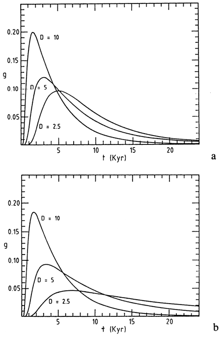
Figure 8a depicts the probability density g(z, t) for reaching the boundary starting at z = 0 for three different values of D. We observe a dispersion of passage times measured by the variance <δt2>, which is comparable to the mean and gets increasingly large as D (or q2) gets small. However, the normalized dispersion <δt2>1/2 / <t> is less sensitive to the variations of D. An interesting manifestation of the role of stochastic effects is that the probability density attains its maximum at a value of time that is less than the deterministic time ![]() = 1/v0. This result suggests that one should be extremely careful before adopting the usual (linear) correspondence between the elapsed time and the depth of a sediment. Notice that for fixed values of D and v0 the shift of the maximum relative to t becomes less pronounced as the size of the system increases.
= 1/v0. This result suggests that one should be extremely careful before adopting the usual (linear) correspondence between the elapsed time and the depth of a sediment. Notice that for fixed values of D and v0 the shift of the maximum relative to t becomes less pronounced as the size of the system increases.
Figure 8b depicts the probability density g(z, t) when the drift velocity is negligible. We observe that for large values of D the difference with the preceding case is rather small.
Figure 8--Probability density g(z, t) computed from Eq. (19) for reaching a given depth of the sediment z = l starting at z = 0 for three different values of D in cm2/k.y. Parameters used l = 10 cm. (a) v0 = 1 cm/k.y.; (b) v0 ≈ 0.
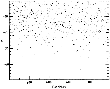
Let us now turn to the distribution of arrival depths at a given time. Figure 9 depicts the results of a numerical simulation of the stochastic dynamics involving N = 1,000 realizations, each starting on the surface z = 0 and running over 10 k.y. We again obtain an appreciable dispersion because, for one thing, in the absence of fluctuations and for v0 = 1 cm/k.y. all realizations should be at depth z = 10 cm.
Figure 9--Distribution of arrival depths at t= 10 k.y. deduced from numerical simulation of Eq. (16) involving 1,000 particles starting at z = 0. Parameter values as in fig. 8a with D = 5 cm 2/k.y.
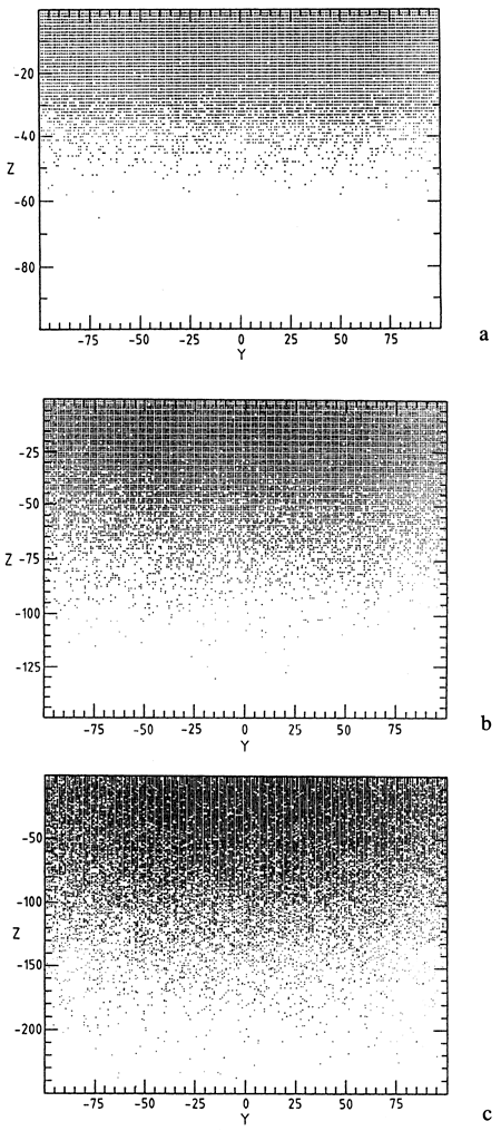
We have extended these studies to a two-dimensional medium and have found that the presence of a second (horizontal) direction adds completely new features. Specifically, as shown in fig. 10, a fractal diffusion front separating a region of densely occupied sites from a region of sparse occupation appears (Feder, 1988). The front has a complex irregular form in space and broadens as time advances. It thus becomes increasingly difficult to predict in an unambiguous manner which characteristic depth will be reached in a given lapse of time. As a corollary, trace deposits on two horizontal layers at different depths could correspond to a chronologic order that is different from or even opposite to the one suggested by sheer inspection of the depths.
Figure 10--Spatial distribution of 50,000 particles performing a random walk in a two-dimensional lattice initially at z = 0 and -100 ≤ y ≤ 100 after (a) t=500, (b) t=2,000, and (c) t= 8,000 time steps. Note the high degree of fragmentation of the front and the increase of its width with time.
We have seen that dynamic systems theory provides us with interesting insights into the variability of our natural environment. We have pointed out that the unstable character of the dynamics of the principal atmospheric and climatic variables entails the existence of an intrinsically generated, irreducible complexity that can in no way be attributed to incomplete knowledge or to the large number of variables and parameters involved. Furthermore, we suggest that, in view of the structural complexity of geologic materials, the correspondence between sediment depth and time history may be far more intricate than a simple one-to-one relationship.
It is our hope that the ideas set forth here will contribute to the awareness of geoscientists about the usefulness of nonlinear dynamic systems both as a source of inspiration for new ways of looking at sometimes long-standing problems and as a quantitative tool of primary importance in the art of modeling and forecasting.
This work is supported in part by the Epoch program of the Commission of the European Communities and the Global Change program of the Belgian government.
Baker, G., and Gollub, J., 1990, Chaotic dynamics: Cambridge University Press, Cambridge, 182 p.
Benzi, R., Parisi, G., Sutera, A., and Vulpiani, A., 1982, Stochastic resonance in climatic change: Tellus, v. 34, p. 10--16
Bergé, P., Pomeau, Y., and Vidal, C., 1986, Order within chaos: Wiley, New York, 179 p.
Berger, A., ed., 1981, Climatic variations and variability--facts and theories: Reidel, Dordrecht, 795 p.
Boudreau, B.P., 1986, Mathematics of tracer mixing in sediments--spatially dependent diffusive mixing: American Journal of Science, v. 286, p. 181-198
Demarée, G. R., and Nicolis, C., 1990, Onset of Sahelian drought viewed as a fluctuation induced transition: Quarterly Journal of the Royal Meteorological Society, v. 116, p. 221-238
Feder, J., 1988, Fractals: Plenum, New York, 283 p.
Feller, W., 1968, An introduction to probability theory and its applications, v. 1: Wiley, New York, 509 p.
Gardiner, C., 1983, Handbook of stochastic methods: Springer-Verlag, Berlin, 442 p.
Grassberger, P., and Procaccia, I., 1983, Characterization of strange attractors: Physics Review Letters, v. 50, p. 346-349
Guckenheimer, J., and Holmes, P., 1983, Nonlinear oscillations, dynamical systems and bifurcations of vector fields: Springer-Verlag, Berlin, 459 p.
Mandelbrot, B., 1977, Fractals--form, chance, dimension: Freeman, San Francisco, California, 365 p.
Nicolis, C., 1982, Stochastic aspects of climatic transitions--response to a periodic forcing: Tellus, v. 34, p. 1-9
Nicolis, C., and Nicolis, G., 1981, Stochastic aspects of climatic transitions--additive fluctuations: Tellus, v. 33, p. 225-234
Nicolis, C., and Nicolis, G., 1984, Is there a climatic attractor?: Nature, v. 311, p. 529-532
Nicolis, C., and Nicolis, G., 1986, Reconstruction of the dynamics of the climatic system from time series data: Proceedings of the National Academy of Sciences USA, v. 83, p. 536-540
Nicolis, C., and Nicolis, G., eds., 1987, Irreversible phenomena and dynamical systems analysis in geosciences: Reidel, Dordrecht, 578 p.
Nicolis, G., and Prigogine, I., 1989, Exploring complexity: Freeman, New York, 313 p.Rössler, D., 1979, Continuous chaos-four prototype equations: Annals of the New York Academy of Science, v. 316, p. 376-392
Shackleton, N. J., and Opdyke, N. D., 1973, Oxygen isotope and paleomagnetic stratigraphy of equatorial Pacific core V28238--oxygen isotope temperatures and ice volumes on a 105 and 106 year scale: Quaternary Research, v. 3, p. 39-55
Wong, P. Z., 1988, The statistical physics of sedimentary rock: Physics Today, December, p. 24-32
Kansas Geological Survey
Comments to webadmin@kgs.ku.edu
Web version March 12, 2010. Original publication date 1991.
URL=http://www.kgs.ku.edu/Publications/Bulletins/233/Nicolis/index.html