![]()
Prev Page--Sedimentation || Next Page--Conclusions
Exploration Techniques
Qualitative Well-log Analysis as an Aid to Exploration
Most wells in the study area have been logged and well cuttings are available. Cores are limited in number, but, where present, assist greatly in the interpretation of samples and logs. Exploration for oil and gas requires the integration of these types of data in order to establish favorable trends of potential reservoir rock units.
General trends in composition of the alternating shales and limestones in the Lansing and Kansas City Groups are discernible from geophysical well logs, provided that comparisons of the logs with cores are available for parts of the area (Figs. 7, 8). The log responses indicate sharper transitions between dissimilar rock types in a southward, or basinward, direction. Having identified the various members of cyclic zones in cores of several wells, it has been possible to recognize compositional variations in these zones on the basis of graphic cross-plots of log values from Gamma Ray (GR) versus Neutron (N) logs (Figs. 38, 39). The relative positions of groups of data points representing different kinds of units in the cycles suggest that such plots may be used to differentiate between the units in cases where identification is in doubt and no core is available. This may aid in correlating logs, in recognizing the appearance of additional limestones in the vertical sequence, and in mapping compositional change of the rocks as an indication of basin shape and direction to sources of terrigenous sediment. For instance, some of the lower intervals of regressive carbonate units are more distinct, on the logs, from underlying marine shales in a basinward well than in a more northern, landward well (Fig. 38).
Figure 38--Cross-plots of gamma ray-neutron well log readings for each of six different Lansing-Kansas City cycles. Rock facies are identified by core-well log correlation. Clusters of points representing five different facies are identified by individual patterened areas. An empirical porosity index is placed along the neutron axis. Each plot represents data from an individual well. A. Typical of a basinward well with good contrast between facies.
B. Represents a landward well, where influx of clastics was high.
C. Another landward well east of (b), where clastics were somewhat less important.
Figure 39--Gamma ray-neutron cross-plots for six cycles from the Prentics #1 well. Areas that include phylloid algal regressive and transgressive carbonates, D- and E-Zones, respectively, are identified in the figure by D and E.
The regressive carbonates become more distinct and well developed basinward due to a decreasing clastic component. Some of the lower regressive carbonates in the Adell well are distinctly denser carbonate than occur landward (low GR and high neutron cps). Marine shales in a more basinward position commonly have a distinctly higher GR response (200 API units) than that of the average shale base line. Northward, the GR response of the marine shales progressively decreases and becomes more like that of the regressive shales. Northward, all the facies tend to converge toward the regressive shale position depending on the abundance of clastic influx throughout the cycle.
According to the epeiric sedimentation model described earlier, the period of marine-shale deposition was longer farther basinward than it was landward, and the sedimentation rate was lower basinward. X-ray diffraction and core description suggest marine shale can be distinguished from regressive shales because of the higher carbonate content and greater clay fraction (Watney, 1979). Probably the lower intervals of regressive limestone units are more distinct from marine shales in basinward areas because they are less argillaceous, more dense, pure limestones. There was not the almost continual influx of terrigenous sediment in basinward areas that there was farther landward. Slower basinward clastic sedimentation and reducing redox potential during burial with organic matter preservation also would have resulted in the enrichment of marine shales in heavy metals and possibly uranium, which would have caused an increase in their radioactivity.
Specific carbonate facies can be identified in the cross-plot in conjunction with limited core information. A plot of six cycles in the No. 1 Prentice well distinguishes the relatively clean, but low-porosity, portion of the phylloid algal carbonate of the D-Zone carbonate from the other regressive carbonates (Fig. 39). Similarly, the phylloid algae-bearing transgressive E-Zone is distinguished on this plot from the other transgressive carbonates. The porous upper regressive carbonate grainstone-packstone of G is identifiable on the plot (low GR-N).
The cross-plots (Figs. 38, 39) do show distinctions among the facies; the positions of various units on the plots do appear to be a function of their location in the basin. Nevertheless, the overlap of some plots and the imprecision of the technique demonstrates the importance of cores and samples in providing specific identifications of facies. It is not possible to interpret and map accurately the detailed changes of facies with only data from well logs. This technique is appropriately used as a reconnaissance tool. It provides another insight into basin development by illustrating the differences and similarities of the cycles within and between wells. The technique does not preclude other conventional forms of analysis, but complements cross-section and isopach studies.
Quantitative Well-log Analysis as an Aid to Exploration
Another method of exploration that may be useful for suggesting trends of potentially porous reservoir rocks in the study area and farther south is the use of quantitative log analysis to map trends of thickness and porosity, and of estimated oil saturation of individual prospective limestones. The present study offered the unusual opportunity to examine various log-evaluation techniques in comparison to core analysis data. This resulted in recognition of some pitfalls of which the geologist must be aware, and of graphic techniques that maximize the utility of log-derived information in sparsely drilled areas, especially where cores are also available.
Thickness--The determination of thickness is usually straightforward, but, in working with relatively thin carbonate beds and even thinner porous zones, it is important in mapping small but possibly significant changes to have logs that accurately record these thin intervals. Logging tools with a source-to-detector spacing greater than the interval of interest do not accurately record its thickness. Porosity-recording tools commonly offer good bed definition, but the older, long-spaced resistivity tools do not. A focused resistivity tool, such as a "Guard" or "Laterolog" is excellent in this use, particularly when the ratio of formation resistivity to mud resistivity is high, and formations present a large resistivity contrast. Previous workers (Hartman, 1975) have described the bed resolution capability of types of logs common to the study area.
Porosity--In this study, porosity is derived from several types of logs, including the commonly used thermal-neutron, gamma-neutron, sidewall-neutron, compensated density, and sonic logs. In the absence of other porosity-logging tools, resistivity from a "Microlaterolog" has been used to calculate porosity.
It is common practice to determine the log response corresponding to zero porosity (so called "matrix value") in limestones by cross-plotting readings from sonic and density logs in the same interval. Various inaccuracies arise from using these "matrix values" in the study area, as revealed by observation of cores. The carbonates are quite variable in composition, ranging from clean limestones and dolomites to cherty, silty, and argillaceous carbonates. The "matrix values" typically are derived from the more dense carbonates in the somewhat shaly lower part of the regressive carbonate units. These intervals commonly are not the same type of rock as is being evaluated in the reservoir interval. Consequently, the porosity that is calculated is not correct.
In areas of frequent lateral change in composition where samples or cores are not examined, formations may change undetected from limestone to dolomite. In such a case, "limestone porosity" values calculated from a sonic log are lower than actual porosity of the dolomite. Cherty and silty limestone zones, conversely, would have actual porosities that are less than the calculated porosity. Two porosity devices, though, would allow discrimination between two lithologies or mixtures thereof.
Some allowance or correction for this "shaliness" effect in the carbonates is possible, but the results must be used with care. In a shaly carbonate, with two porosity tools run simultaneously (e.g., density-sonic or density-neutron), the relative abundance of two lithologies (clay and carbonate) can be determined and porosity can be adjusted. Clay increases the apparent porosity, approximately proportionately to the amount of clay present; from this relationship, a correction for porosity vs. clay content can be derived. In attempting to make accurate estimates of clay content of a carbonate, based on GR logs, it must be understood that the clay in the carbonate is probably not the same type of clay as in the adjacent shales, particularly if those are the red-brown, regressive shales. Another difficulty arises from the fact that, as noted above, the marine shales typically have an unusually high GR response; thus, finding a shale base line (100 percent shale) that is appropriate for correcting porosity of limestones for their shale content is difficult.
Another consideration is the apparent radioactivity of some cherts in the study area. The GR response in a chert zone may be nearly as high as that of a marine shale. Some chert samples have scattered specks of fine, organic (?), black material or dark mottling that apparently produce the abnormally high GR responses (Fig. 40). This dark matter is probably organic material with a high uranium or thorium content (Hassan and others, 1976).
Figure 40--Cuttings from the A-Zone identified on this well log contain abundant orange chert with pinpoint-sized, scattered black (organic) material and dark mottling. Note the high GR record and also high neutron and guard log response in the middle of the A-Zone at the position of the arrows. The neutron and guard logs both suggest a nonshaly, tight carbonate interval contrary to the indication of the GR log. (Murfin McCain #1, 7-4S-33W)
The porous zones that are present in carbonate units in the study area usually occur in limestone or dolomitic limestone that is not shaly. Reconnaissance estimates of porosity made in these types of rocks are slightly pessimistic if dolomite is present. Effective porosity is that which represents interconnected pores in the rock. An average threshold, or minimum, porosity can usually be defined above which there is some assurance that the rock is permeable (Fig. 41). In the present study, carbonate units with porosity above eight percent are usually permeable. The high permeability-high porosity samples in both wells represented in Figure 41 have complex, primarily intergranular porosities, with varying amounts of vugs, solution molds, and fractures. The low porosity-high permeability zones are vuggy, fractured lime mudstone, wackestone, or packstone. Good results of drillstem tests of these units correlate positively with trends of higher porosity and permeability as shown on this plot (Fig. 41). Porosity determined separately from analyses of a well log and core (Fig. 6) shows close correspondence between the two techniques, although, in detail, there are differences. The core analysis data are derived from measurements on a one-inch core plug and the log values are actually averages over intervals of approximately two feet.
Figure 41--Semi-log plot of core analysis permeability versus porosity for (a) Skelly Bartosovsky #1 (9-1S-34W) in Rawlins County, and (b) Conoco Adell L-KC Unit 406 (2-6S-27W) in Sheridan County. The increase in permeability with increasing porosity is more evident in the Bartosovsky data set. Generally, rock whose porosity is greater than eight percent is also permeable.
Formation Fluid Saturations--Another difficulty in analyzing logs of the Lansing-Kansas City Groups in the study area for porosity and fluid content is the highly variable degree of cementation that results from the complexity of facies and diagenesis of these rocks. As with any shallow-marine sequence, these rocks vary in composition over short distances, and they have been subject to a variety of diagenetic processes. The experience of operators in the area is that log analysis can be very misleading unless it is complemented with attention to the specific type of rock represented by the logs, i.e., by examination of cuttings or cores. The cementation exponent, m, the formation factor, F, and the formation water resistivity, Rw, are essential in most calculations of porosity and fluid saturation, and these are the very factors that are most affected by the variability of the rocks described here.
The need to know Rw can be circumvented when a sufficient number of values of porosity, ![]() , and true formation resistivity, Rt, is available from logs to construct a plot such as that shown in Figure 42. This plot may also be used to estimate cementation exponent, m.
, and true formation resistivity, Rt, is available from logs to construct a plot such as that shown in Figure 42. This plot may also be used to estimate cementation exponent, m.
This estimation was not made in Figure 42 because of lack of sufficient points representing the water-wet section. The Ro line was calculated on the assumption that the cementation exponent equals two. The equation of the Ro line is:
The positions of water saturation (Sw) lines, 50 percent and 30 percent, are calculated by using Sw = Rt/Ro, where Sw equals 0.5 for 50 percent and 0.3 for 30 percent values of Sw. Rt, the true formation resistivity, is solved for at least values of porosity to construct the water saturation lines.
In the example cited here (Fig. 42), the value of Sw derived from log analysis for the H- and J-Zones corresponds well with the results of core analysis and drill-stem tests. Core observation demonstrates that these two intervals are dominated by granular-type porosity (altered lime-mud) and are low in clay. The sonic log alone provides a good measure of porosity. In contrast, in the A-Zone porosity is developed as a combination of fine granular, vuggy, and fracture development in a shale-laminated, mud-rich carbonate. Even though the core analyses and drill-stem tests indicate oil, the plot suggests high water saturation.
Figure 42--Log-log plot of induction well log resistivity versus shale-corrected sonic porosity for porous zones of Skelly Bartosovsky # 1. Data points determined on a per-foot basis. Carbonate intervals are labeled accordingly. The solid heavy line is the Ro (water wet) line with slope, m (cementation exponent), equal to 2, and with an intercept of 100 percent porosity at 0.07 ohm-m (= Rw ), determined by calculating Rw from SP deflection in porous, water-wet zones. Sonic log porosity was corrected for shale effects with a Dresser-Atlas nomograph (p. 7-1 of Log Interpretation) using the gamma-ray response. The points labeled "B" represent the sandstone-siltstone unit immediately below the A-Zone. The circled K values represent water-wet points, which are best represented by a water-wet line with m = 2, Rw = 0.09 shown in part on the lower right of the plot.
| Drill Stem Test Results (by zone) | |
|---|---|
| Zone | Results |
| J | 3360' oil, SIP: 1305-1280#, FP: 160-1250# SWB 144 BO/2 hrs. |
| H | 2249' gas + 1880' oil, SIP: 1305-1250#, FP: 135-745#, SWB 132 BO/2 hrs. |
| A | 320' gas, 160' oil, SIP: 1280-1120#, FP: 50-80#, SWB 122 BO/2 hrs. |
| G | 3 gallons water/hr. with show oil |
| D | 5' mud with specks oil, SIP: 130-0#, FP: 0-0# |
| K | 60' muddy saltwater with specks oil, SIP: 1330-1120#, FP: 0-0# |
| Abbreviations | |
| SIP: | shut-in-pressure (initial and final) |
| FP: | flowing pressure (initial and final) |
| SWB: | swabbed |
The sonic log does not respond to discontinuous secondary porosity as fractures and scattered vugs. Rather, most of the acoustic energy travels around these disruptions and is not detected with the sonic log. The core analysis porosity values in the lower A-Zone are up to 13 percent, whereas the sonic values are all under 10 percent with the exception of one value. The higher actual porosity would lower the water saturation as the plot demonstrates.
In addition, the shale laminations that are present probably have depressed the induction resistivity response. Shale tends to "short-circuit" a resistivity log by conducting the electrical current around the oil- filled pores and thus to lower the resistivity. Consequently, the apparent water saturation is high.
The B-Zone is a shale-laminated, sandy quartz siltstone. The shale correction that was applied to the sonic log through this interval was substantial. Core analysis porosity values are over 15 percent while the corrected sonic values using a sandstone matrix are noticeably lower (under 10 percent).
The gamma-ray tool apparently overestimates the shale fraction in this zone and the resulting shale corrected porosity is too low. The shale fraction is considered proportional to the gamma-ray reading between that of a shale-free formation (0 percent shale) and the average shale gamma-ray intensity (100 percent shale). This overestimation of shale by the gamma ray is not unexpected as this transgressive unit contains shale similar to the marine shale. Indeed, the gamma-ray response in the marine shale may be quite high, exceeding by several times the average shale gamma-ray value. Thus the gamma-ray value may actually be indicating a lower shale fraction. The presence of the shale has substantially lowered the resistivity values for this interval. Compensating for both of these effects would move the points toward lower water saturation (toward the 50 percent Sw average determined by core analysis).
Log analysis of shale-free reservoirs with intergranular porosity is generally routine, but complex lithologies and pore systems normally require running additional logs, e.g., density or neutron, to complement the logging suite. Similarly, core and core analyses provide pertinent information for understanding the well logs.
The cementation exponent that applies to these formations varies from 2 to 2.8. Useful reviews of this element in the determination of formation factors in carbonate reservoirs are given by Gomez-Rivero (1976), DeWitte (1972), and Chombart (1960). The exponent, m, in the equation, F = 110m, is approximately equal to 2 for most types of pore systems. For oomoldic systems, a type that is common in the Lansing-Kansas City limestones in areas south of the present area of study, m may be as high as 2.8 (Tixier, 1962). The uncertainty in the value of m results in occasional errors in the calculation of F and, consequently, of Sw (Fig. 42). Formation factor, F, may also be estimated from values of resistivity in the flushed zone if a microresistivity log, such as a "Microlaterolog" or "Proximity log," is available.
A useful technique for detecting changes in formation composition and in the nature of formation fluids is the mapping of Rwa, apparent water resistivity, determined by dividing Rt, from a deep-reading resistivity log, by F, derived from a porosity log. Rwa is an indication of variations in water resistivity or cementation exponent (nature of the formation), or of the presence of hydrocarbons in part of the pore space. For this reason, maps of Rwa, when used in reconnaissance of a region with well logs, assist the geologist in recognizing areas where further study, of samples, drill-stem tests, or cores may result in the recognition of apparently anomalous conditions. These areas may be important in the evaluation of prospects for drilling.
Mapping Facies from Well Logs and Samples--Examples from Rawlins County
One good method of defining prospective drilling locations as extensions of known oil-producing areas is to establish trends, in these areas, of factors that are associated with production and that can be mapped. Such a trend could be established simply by recognizing an anticlinal fold, a thin or thick area of the reservoir unit, or a similarity in the values of some parameters calculated from logs, such as rock and fluid properties. The actual significance of such a trend depends, of course, on the density of well control and the number of variables that substantiate the trend.
Potential hydrocarbon reservoir carbonates in the Lansing-Kansas City Groups should be mapped as individual sedimentary units, or elements of the cycles discussed above. The location of oil and gas production, within each major carbonate unit becomes understandable only in this way. Aggregating information for mapping from several zones results in confusion in many cases. It is important to recognize the development and expression of sedimentary cycles in the Lansing-Kansas City and to incorporate these into the strategy of mapping and exploration. Later "stacking" of maps to compare cycles and to understand their underlying causes can be beneficial as a predictive tool in exploration.
Rawlins County, Kansas, which lies on the flanks of the Cambridge Arch (Figs. 2, 4), was selected for detailed logs and cuttings analysis and as a test area in which to construct various maps that might be useful for establishing prospective exploration trends because of earlier studies in the area, the availability of cores from several wells, and the high level of current activity in this part of Kansas and adjoining states. Cumulative oil production in Rawlins County through 1978 amounted to 10.9 million barrels, with 95 percent of the production having come from the complex of larger fields in the northern part of the county (Beene, 1979). This area is referred to as the Cahoj- Wilhelm structural complex and encompasses 16 fields (Fig. 43). The remainder of the production is from 14 fields in central and southern Rawlins County. The most productive area has been Cahoj Field in Township 1S-34W, with oil production from 10 separate intervals.
Figure 43--Structure contour map, top of Lansing (A-Zone carbonate), Rawlins County. Grid system is six-mile square township divisions. Red dots represent well control. This base is the same as that used for all succeeding maps. Because of the inadequacies in some of the data, not all points of control are used on each map.
Mapping that would suggest reasons for the locations of the various oil reservoirs and whether they are mainly structural, stratigraphic, or a combination of the two was completed for several cyclic units (Pl. 1). The sedimentary cycle including the J-Zone was examined initially, as it currently is the most productive unit in Rawlins County. For comparison, a stratigraphic analysis was also made of the overlying H-, G-, and D-Zone Cycles. Significant variations in the character of these units have been interpreted in terms of differences in their mode of deposition and the geologic events that have subsequently affected them.
J-Zone Cycle--The J-Zone is the "upper" or "regressive" carbonate unit in the cycle of genetically related units referred to here as the "J -Zone Cycle" (Fig. 44). The structural shape of the top of the J -Zone (Fig. 45) clearly does not account for the distribution of all the oil production from this reservoir. Production is obviously localized on-structure in some areas, such as the Cahoj structural complex; but, in others, production is confined to the flanks of positive anomalies.
Figure 44--Definition on gamma ray-neutron logs of intervals depicted on isopach maps that follow. Intervals are defined and labeled on the appropriate log curve. Note the overlapping interval of the marine shale (defined by the gamma ray log) and regressive carbonate isopach interval (defined by the neutron log).
Figure 45--Structure contour map, top of J-Zone carbonate, Rawlins County. These are estimated from minimum oil/water (min o/w) contacts estimated from well logs. The smaller nonporous areas are omitted from the productive areas over Cahoj and Wilhelm fields. The minimum o/w's vary from -1905 to o-1160, a range of 65 feet.
Reconnaissance maps of J-Zone in Rawlins County, prepared solely with data from well logs, give some indication of the importance of factors other than structure that may be significant in forming oil traps (Figs. 46, 47). The thickness of J-Zone with effective porosity greater than eight percent, expressed as thickness times porosity (Fig. 46), gives some indication of the attractiveness of the zone as a target for exploration. Recognition from logs that most of the porosity is in the upper parts of the limestone suggests that the sedimentary models discussed earlier may be useful in explaining its origin. Elongate trends of greater porosity occur with no apparent relationship to structure in some areas. An understanding of these features depends on analysis of other kinds of information.
Figure 46--Contour map of porosity exceeding eight percent in the J-Zone carbonate in Rawlins County. Porosity is multiplied by the average thickness of the porous interval. Three separate contour sets identify porosity developed inthe upper, middle, and lower portions of J-Zone. Highest frequency of occurrence of porosity is in the upper interval of this regressive carbonate in the more shallow-water carbonate facies. Rock with porosity exceeding eight percent is usually permeable.
Figure 47--Map of the apparent water resistivity (Rwa) of the upper J-Zone carbonate in Rawlins County, derived solely from well-log data. Rw. = Rt/F where Rt is the reading from the deep-investigating resistivity tool and F is the formation resistivity factor defined as I/(Porosity)m, m = 2. Note that m = 2 is assumed (Fig. 42) and, as indicated in the text, the cementation exponent may be highly variable. A real difference in cementation and tortuosity of pores may account for some of the variation in Rwa over the map area.
Another type of map that is derived from well-log analysis is the map of apparent water resistivity Rwa (Fig. 47). As indicated above, this parameter may reflect a number of variables; but the correspondence of slightly higher Rwa values with trends of greater porosity (Fig. 46) and of oil production (Fig. 45) in the J-Zone suggests that these higher values may relate to hydrocarbon saturation. To confirm this, it would be necessary to do additional studies on the lithology of samples (degree of cementation) and to refine estimates of porosity from logs with corrections for shaliness. The usefulness of this type of map is not yet established in this area. Other maps that are derived from logs, but that can be combined with information from studies of drilling samples or cores to understand the patterns that appear, are maps of the thickness of genetically related units of the J-Zone Cycle (Figs. 48, 49). Reference to Figure 44 indicates the intervals discussed below.
Figure 48--Marine-interval isopach, J-Zone cycle, Rawlins County, derived from porosity or resistivity log includes the top of regressive carbonate to the base of the transgressive carbonate (Fig. 44). Note that the 16- and 20-foot contours are added to this isopachous map. Marine shale isopach is defined from the interval identified on a gamma-ray log, as shown in Figure 44. This method commonly includes a portion of the lower, argillaceous, regressive carbonate.
Figure 49--Regressive shale isopach interval, defined by gamma-ray logs as in Figure 44. Regressive carbonate isopach derived from porosity log or resistivity log, as shown in Figure 44. Lower portion of carbonate may appear as shale on the gamma-ray log. Note addition of 12- and 16-foot contours.
Definition of the marine shale unit with the gamma-ray log results in inclusion of the shaly lowermost part of the regressive limestone (Fig. 44) with the dark radioactive shale in mapping this unit. In most areas the marine shale is fairly thin and uniform in thickness. Nevertheless, there are many isolated areas of marine-shale thickening in Rawlins County that can be directly attributed to thickening of the shaly regressive carbonate. This local thickening of the shaly fraction of the cycle is probably due to an early onset of carbonate mud accumulation.
The seafloor bathymetry and or bottom currents may have been important factors influencing this onset of regressive carbonate deposition. This idea will continue to be supported in the following discussion.
Trends of thickening of the J-Zone, or regressive, carbonate (Fig. 49) occur both north and south of a central east southeast-west southwest trend of thinness. Lithofacies (Fig. 50) of this J-Zone carbonate indicate that the thicker area in the north consists mainly of peloid, lithoclast, and skeletal grainstones that have undergone freshwater diagenesis; but the thicker area in the south (Fig. 49) is mudstone or wackestone with less evidence of early leaching and disruption. This relationship suggests that the southward thickening reflects the basinward direction from an area of northern nearshore shoals or supratidal deposits. The central area of thinner section was probably an area of slower sedimentation between shoals at the time of deposition, where only a few scattered, current-winnowed grainstone and packstone deposits formed. Increasingly restricted water circulation is indicated by less diverse assemblages of fossils in the deposits of these inter-shoal areas.
Figure 50--Carbonate facies map of the upper portion of the J-Zone in Rawlins County. Thirty-seven sample-control points, supplemented by isopachous maps, provide identification of facies. Facies consist of a simple series of skeletal grainstone shoals, including a variety of grain types among a more extensive area of mudstone-wackestone, identified by the open areas on this map. The areas of occurrence of the grain-supported rocks are probably more complex than shown here. The packstone fringe represents a zone of gradation between the high- and low-energy deposits.
The Cahoj-Wilhelm structural complex probably was a positive area during the Pennsylvanian; and it affected patterns of sedimentation in northern Rawlins County, Kansas, and north of there in Nebraska at that time. Concentration of grainstone deposits on its flanks or crest in several depositional cycles and evidence of subaerial weathering and dolomitization of the carbonate units and paleosoil formation in overlying regressive shales (Watney and Ebanks, 1978) support this idea. This important early diagenesis in the J-Zone carbonate has resulted in its becoming the most porous and permeable reservoir in Cahoj Field, despite the fact that originally much of the J-Zone was a lime mud-rich sediment and, probably, impermeable.
These conclusions are supported by isopach maps of the marine interval (Figs. 44, 48) and of the regressive shale unit (Figs. 44, 49). These two mapping units tend to be complementary in thickness and to reinforce the idea that the regressive shale thins basinward from a northern source of terrigenous clastics. The regressive shale fills in the depositional relief on the underlying regressive carbonate. This same relationship occurs in other cycles of the Lansing-Kansas City section.
Isopach and lithofacies maps, when combined with maps of porosity and other log-derived parameters, can be interpreted in terms of the geologic history of a potentially porous carbonate reservoir rock. Trends of grainstones with intergranular porosity or packstones and originally impermeable wackestone or mudstone deposits with secondary porosity can be mapped as they are encountered during drilling if the general basin geometry and sedimentation patterns are known. Knowledge of what trends and patterns are significant in any exploration area can be gained only by integration of information from logs and samples or cores. Examples from other cycles of sedimentation in the Lansing-Kansas City Groups strengthen this conclusion, and they illustrate the fact that there are many facies in Lansing-Kansas City carbonate zones, other than those described from the J-Zone, which should be considered in a regional exploration play.
H-Zone Cycle--The sediments of this cycle may be the product of deposition in deeper, more basinward conditions than those of the J-Zone Cycle, and, as such, may indicate the type of facies that would also be present in J-Zone Cycle south of the study area. Broad trends of facies, tens-of-miles wide, may be present in these deposits, as demonstrated by studies in eastern Kansas (Heckel, 1975).
The "transgressive," or "lower," limestone of the H-Zone Cycle (H') in Rawlins County (Figs. 44, 51) is thicker and more easily measured on well logs than is the equivalent unit in the J-Zone Cycle (J') (Fig. 44). Thicker areas in this unit correspond well with general areas of thicker "marine interval" (Figs. 44, 51). The "regressive" carbonate (H-Zone) of this cycle (Figs. 44, 52) also is thicker where the marine interval, overall, is thicker. These thicker trends of H-Zone (Fig. 52), particularly in northernmost and southern Rawlins County, with a thinner area between, are similar to, but more pronounced than, trends in the J-Zone.
Figure 51--Transgressive carbonate isopach and marine interval isopach, H-Zone cycle, Rawlins County. Marine interval defined on log in Figure 44. Note addition of 22-foot contour.
Figure 52--Regressive shale and regressive carbonate isopachs, H-Zone cycle, Rawlins County. Regressive-carbonate isopach interval is defined on log in Figure 44. Note addition of 12- and 16-foot contours.
Trends of change in thickness of the "regressive" shale above H-Zone (Figs. 44, 52) are complementary to those in the underlying carbonate. Because it is unlikely that a red-brown shale such as this would interfinger with a marine carbonate unit such as the H-Zone, the thinning of the shale probably indicates the presence of carbonate build-ups, that is, areas that had some relief at time of deposition.
Lithofacies of the H-Zone carbonate (Fig. 53) are more varied than those of the J-Zone, and they suggest a reason for the local thickening of this unit in southern Rawlins County. Fragments of phylloid algae (Fig. 8) are abundant in samples and cores of H-Zone in wells located near the areas labeled as mud banks on Figure 53. These algal banks evidently are similar to those in eastern Kansas (Wilson, 1957; Harbaugh, 1959; Heckel and Cocke, 1969), and, perhaps, to others in areas where they are important oil reservoirs (Elias, 1962; Choquette and Traut, 1963; Wilson, 1972; and Wermund, 1975). These banks probably formed on an open-marine shelf where there was good light penetration through clear water. Fragments of a diverse assemblage of fossils and the sparse terrigenous silt or mud in these sediments support this idea. Occasionally, strong currents winnowed and sorted the bioclastic grains on these banks, and formed lenses and layers of skeletal sand, especially on the flanks of the banks. Heckel and Cocke (1969) have reported other types of coarse carbonate deposits, tidal channel-fill, spits, and bars, associated with algal banks.
Figure 53--Carbonate facies map of upper regressive H-Zone carbonate. Cuttings and core control points labeled. Facies include a thick phylloid algal-mudbank and a grainstone shoal, separated by areas of skeletal lime-mudstone-wackestone. Divisions shown within packstone facies separate areas in which the types of skeletal particles are different.
The algal-bank facies of the regressive carbonate, H-Zone, has not yet proven to be productive of oil and gas, mainly because there is insufficient porosity and permeability. The limited diagenesis that this facies has undergone has not enhanced the properties sufficiently. Other carbonate zones (e.g., D-Zone) in this area that have similar facies appear to be more favorable as reservoir rocks.
The only production of oil and gas from H-Zone has been from grainstone facies in the Cahoj area, northern Rawlins County, where prominent carbonate shoals were formed by waves and currents acting on the pre-existing bathymetrically high area (Figs. 40, 53). Figure 54 is a photomicrograph of a representative cutting from this grainstone facies.
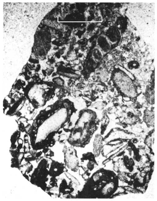
Figure 54--Thin section photomicrograph of cuttings sample from the Skelly Cahoj D-1 (17-1S-34W), located in an area of grainstone shoal facies of the H-Zone carbonate at Cahoj Field. Predominantly a coarse-grained, crinoid, bioclastic grainstone with scattered brachiopods, small bivalves, and forams. Encrusting forams common. Occasional quartz silt grains present. PLANE-POLARIZED LIGHT. Bar scale equals 1 mm.
The regressive shale and siltstone that eventually blanketed H-Zone had less influence on carbonate sedimentation than did their counterparts in the J-Zone Cycle. Thick areas of this silty facies are restricted to locations north and northwest of the Cahoj complex (compare Figs. 50 and 53).
G-Zone Cycle--The isopach intervals of the G-Zone cycle illustrate another facet of cycle development. Although the "transgressive" limestone (G') (Fig. 55) is relatively thin throughout the area, it gradually thickens to the south. The marine interval (Fig. 55) noticeably thickens in the north and central areas of Rawlins County, the latter location along a trend just to the north of the H-Zone Cycle marine interval and carbonate thicks (Figs. 51, 52).
Significantly, the marine interval in the G-Zone Cycle thickens over Cahoj Field without a complementary regressive carbonate thick as found in the northeast and central areas of Rawlins County (Figs. 55, 56). In other areas, the regressive shale thinning complements the thickening of the underlying regressive carbonate (Fig. 56) and suggests depositional relief in these areas analogous to that described in the H-Zone Cycle. This clastic interval thickens in the northwest, like that of the regressive shale in the H-Zone Cycle (Fig. 52), and in the southwest.
Figure 55--Transgressive carbonate and marine interval isopach, G-Zone cycle, Rawlins County. Marine interval thickness is dominated by marine shale to northwest and regressive carbonate over the remaining area. Cross section in Plate 1, defined by index line D-D' on map, illustrates change from clastic-dominated marine interval of G-Zone cycle in north to carbonate-dominated in the south. Note addition of 34-foot contour.
Figure 56--Regressive shale and regressive carbonate isopachs, G-Zone cycle, Rawlins County.
Limited sample data of the G-Zone regressive carbonate indicate lithofacies variation between areas. The lithofacies interpretation again aids in the explanation of the isopach map trends. The abundant silty-shale laminations throughout the thin regressive carbonate at the Bartosovsky #1 well location (Fig. 56) reflect the turbidity during carbonate deposition. The thick marine shale in the well also shows the importance of the clastic component in the marine interval (Fig. 55) at this location.
In contrast to this clastic-dominated sequence to the north, the No. 1 Prentice core (Fig. 56), located along the north flank of a thickened regressive carbonate, contains phylloid algae and abundant fossils within a relatively clean regressive carbonate. The marine shale interval is correspondingly thin at this location and is substantially less important in the overall marine interval south and eastward from this location. The cross sections along D-D' (Pl. 1) illustrate this facies variation in the G-Zone Cycle.
The phylloid algal-bearing G-Zone carbonate in the No. 1 Prentice well is capped by a subaerial crust. Beneath the crust the carbonate shows evidence of leaching by freshwater. The unit, although porous, is water wet at this location. Similar facies in the G-Zone that have undergone freshwater dissolution may prove productive.
Production is now limited to the northern Cahoj structure complex in grainstone and freshwater-altered packstone and wackestone carbonate reservoirs. Grain-rich carbonates are also present south of Cahoj, including the upper regressive carbonate in the No. 1 Prentice well. G-Zone prospects may invoke either or both types of reservoir rocks: secondary porous algal carbonate and primary porous grainstone.
D-Zone Cycle--The uppermost cycle examined is described by an isopach map of the E-Zone carbonate, the transgressive unit of the D-Zone Cycle (Fig. 57), and a generalized isopach of the regressive D-Zone carbonate (Fig. 58) annotated with lithofacies data from core and cutting descriptions.
Figure 57--Transgressive E-Zone carbonate isopach, D-Zone cycle, Rawlins County. Cross sections along D-D' (Pl. 1) illustrate the thick central east-west trend attributed to phylloid-algal carbonate buildup.
Figure 58--Regressive carbonate isopach, D-Zone cycle, Rawlins County. Productive areas are outlined in the map. Southward thickening is evident in cross section D-D' (Pl. 1). Note limited well control.
The transgressive carbonate (Fig. 57) increases in thickness from only two to 16 feet along a narrow east-west trend in central Rawlins County. This trend directly overlies the G-Zone carbonate thick (Fig. 56) and lies slightly north of a superjacent D-Zone carbonate thick (Fig. 58). Significant local thickening also develops over Cahoj Field.
The D-Zone carbonate isopach map (Fig. 58), gradually thickening to the south, is interrupted by a thicker trend in central Rawlins County as mentioned above. Core and sample data from this carbonate on either side of this thick area contain abundant phylloid algae just as in the H- and G-Zone carbonates. The thicker carbonate probably represents a local proliferation of phylloid algae. Flank areas, although containing phylloid algae, do not necessarily result in thick carbonate development.
The transgressive E-Zone carbonate locally thickens in a pattern similar to the D-Zone development. The thickening is also attributed to the presence of phylloid algae, the first occurrence recognized in this area of algae in the transgressive carbonate. Interestingly, the E-Zone in the Holmdahl #1 core (Fig. 58) in eastern Rawlins County contains a thin, silty, Osagia packstone base; the shoal-water facies is overlain by 3.5 feet of mudstone-wackestone unit, containing phylloid algae in the bottom half foot. In contrast an E-Zone core from the buildup area (Prentice No. 1, 12 feet thick) contains 10 feet of phylloid algal-bearing carbonate (Fig. 11), clearly the dominant facies in this carbonate buildup. During transgression, the carbonate buildup was able locally to maintain more clear shallow-water characteristics by keeping pace with sea-level rise and was not overwhelmed by clastics in prelude to the deposition of the overlying marine shale. Cross sections in Figures 45 and 46 illustrate this carbonate buildup centered near the Prentice No. 1 well.
In contrast, just to the north over Cahoj Field the E-Zone (Fig. 57) thickened through the accumulation of shoal-water grainstone and packstone. The higher sea floor over the Cahoj location was apparently a focus for the winnowing and accumulation of the lower, early transgressive carbonate. The influx of clastics from the north though, during lower energy conditions present during later transgression, precluded phylloid algal development.
Oil production in the E-Zone occurs in only small areas over Cahoj in the grainstone-packstone facies (Fig. 57). Similarly, in the D-Zone carbonate, this facies is productive over Cahoj and in central Rawlins (Atwood Field) near the crest of the carbonate buildup (Fig. 58).
The phylloid algal wackestone facies of the middle and lower D-Zone is locally productive in Happy and Seberger fields located off the north Hank of the buildup in northwest Rawlins County (Fig. 58). The secondary pore space in this algal wackestone is exemplified in the No. 1 Prentice well. Here the D-Zone core contains a 10-foot interval of vugs and fissures, including molds of algae, the result of freshwater leaching and stabilization of this carbonate. The pore space of the upper four feet is filled with graded and laminated deposits of quartz siltstone and very fine grained sandstone (Fig. 17); the deposits closely resemble the overlying clastic sequence. Percolating meteoric waters probably transported this internal sediment down through the carbonate while the unit was subaerially exposed in the vadose zone. Oil-filled porosity underlies the silt-occluded pores. The contact between these may represent the water table at the time of silt infiltration. The pore space below this paleo-water table was saturated with either slow-moving or stagnant water, conditions under which silt could not be transported.
The Prentice No. 1 well produces 16 BOPD from the interval of freshwater-leached, secondary porosity, but in the Frisbie No. 1 well one and one-half miles to the north this same interval had an initial potential of 168 BOPD.
Summary--The four sedimentary cycles have been described through a series of reconnaissance, isopach, and lithofacies maps. Trends of thicks and thins were initially recognized on the reconnaissance and isopach maps. Sample data derived from study of cores and cuttings of the regressive and transgressive carbonates were used to construct lithofacies maps and to describe further these trends.
The reservoir facies of the regressive carbonates in these four cycles are of three types: 1) grainstone and packstone facies, 2) freshwater-leached phylloid algal mudbanks accompanied by flanking or capping grainstone-packstones, and 3) diagenetic, secondary porosity affecting all carbonate rock types. Table 5 describes the various map characteristics used in defining these reservoir facies.
Table 5--Map characteristics that are useful for identifying reservoir facies.
| 1. Grainstone and Packstone Facies | |
| Marine Shale Isopach: Thickening over are of suspected batymetric relief where concentrations of grain-rich carbonates commonly occur. | |
| Regressive Carbonate Isopach: Thickening or thinning depending on winnowed or accretion accumulation. | |
| Marine Interval Isopach: Local thinning common along south flanks of high-energy shoal (e.g. J-Zone Cycle) | |
| Regressive Shale Isopach: Closed local areas of thinning may indicate positive locations while unit was deposited. | |
| Porosity-feet Map: Porosity development at or near the top of the carbonate is a positive indication of grainstone. | |
| 2. Phylloid-Algal Mudbanks with Flanking of Capping Grainstone-Packstone | |
| Marine Shale Isopach: Probable thickening over area of nucleating algal mudbank. | |
| Regressive Carbonate Isopach: Substantial thickening, generally 2x surrounding area; five to ten miles in length. | |
| Marine Shale Isopach: (same as marine shale) | |
| Regressive Shale Isopach: Substantial thinning over buildups. | |
| Porosity-feet Maps: Porosity at any level in the buildup | |
| 3. Early Diagnostic Second Porosity | |
| (in Cahoj area): Thinning or thickening of both regressive carbonate and shale accompanied by associated facies variation (winnowed, silty deposits or thick restricted-marine facies over bathymetric high; focus for early diagenetic processes). | |
| (in phylloid algal buildups): Local thickening of all intervals except regressive shale; (aragonitic algae very unstable during freshwater diagenesis; topographic relief also tends to focus these early diagnetic processes on the buildup). | |
| (in association with high-energy carbonate): Look for map properties as described earlier (primary porosity is potential avenue for movement of diagnetic waters; secondary porosity trends may follow mapped grainstone trends). | |
The Cahoj structure in north-central Rawlins County was a positive feature during the deposition of the Lansing-Kansas City cyclic sediments. Evidence presented here of bathymetric relief over Cahoj conforms to deeper subsurface control that indicates a history of positive relief, including basement faulting (Cole, 1976). Isopach and lithofacies maps illustrate lateral cyclic variation over this feature, which relates closely to the Lansing structural configuration. Grainstone and packstone were frequently developed over and along theflanks of Cahoj. Carbonates in which faunal constituents are restricted and that have been altered by freshwater also are abundant on this feature.
The Cahoj structure is producing in 10 different horizons from both primary and secondary porosity. Seventy percent of the Rawlins County production is obtained from this area (Beene, 1979).
Oil fields south of Cahoj in Rawlins County are smaller and more typical of the immediate area. Although not conforming to present structure as in the Cahoj area, favorable facies with primary and secondary porosity are mapped, such as the grainstone facies in J-Zone and the phylloid algal facies of D-Zone. Evidence from isopach maps suggests subtle bottom relief or slope changes were present at the time of sedimentation across southern Rawlins County.
Mapping the structure from subsurface data indicates production does not always exist on structurally high areas with closed contours. Similarly, present structure may not have any relationship to porosity pinchout. Therefore it is necessary to accompany maps of structure, present production, tests, and log-analysis data with isopach and facies maps. A prospect can then be recommended on the basis of a number of significant criteria.
To the south, beyond the study area, additional carbonate units and changes in the extent of transgression and regression will modify the stratigraphic framework and may change the significance of certain isopachs. Nevertheless, the use of the sedimentary model and the reliance on good samples should allow facies description and the discrimination of potential petroleum reservoirs.
The cycle would be expected to include more marine characteristics and the carbonate-to-clastic ratio should increase, as the cross section A-A', Figure 5, demonstrates. In places the marine shale or regressive shale may be missing entirely. As suggested by the stratigraphic model (Fig. 37) the regressive shale grades basinward from continental to increasingly marine in character, including additional carbonate units. Accordingly, the complementary nature of the regressive shale and the regressive carbonate may not exist. Rather the regressive shale may drape evenly over the underlying carbonate.
Grainstone deposits and mudbanks similar to those observed here persist southward (basinward) as previous studies and experience indicate. The thickness and constituents of the carbonates will vary, though, according to changes in water circulation, rates of deposition and subsidence, and water depth.
Early diagenesis is less extensive and intense in the southern portion of the study area. Similarly, the intensity of early diagenesis should continue to diminish basinward, but the effects may still be locally significant in formation of porosity. For example, the oomoldic zones in the southerly shelf area of Haskell County, described by Brown (1963), probably occurred during early partial dissolution of unstable aragonitic oolites as a response to flushing by undersaturated waters (brackish or fresh). Notwithstanding the general decrease in intensity of early freshwater diagenesis to the south, diagenesis should be important across much of the shelf.
Drilling prospects may be recognized that originated differently but now are adjacent to each other, such as the grainstone trend over and around Cahoj, and porous, altered wackestone within the algal mudbanks of the H-Zone. Structural mapping alone would not detect the latter development. Knowledge of facies with the aid of the structure would be decidedly useful in indicating the potential step-out locations during field development.
Composite isopach maps of more than one carbonate unit in several sedimentary cycles may not reveal these types of trends. The added thickness of adjacent units may mask the important changes within an individual unit. If carbonate buildups in a vertical sequence offset one another, a composite isopach map may indicate only a nebulous thick area, with no clear delineation of prospects.
The task of defining genetic units of a cycle requires time and an understanding of the stratigraphy, but the rewards are apparent. Methods of saving time are available, such as establishing a computer data base, as used here, which can be updated and retrieved on a routine basis. New well data can be placed on punched cards or into a tape file and then posted or mechanically contoured on a new base map with the original data set.
Good samples and core have inestimable value in an integrated approach such as this. The required knowledge of the stratigraphy can only be gained through detailed sample observation. Whether it is referred to as "ground truth" or "back-to-basic geology," this critical step of examining the rocks is essential.
In exploration, well logs are generally used to correlate and pick stratigraphic data. Quantitative well-log analysis is equally important in an exploration program. Resistivity-porosity cross-plots and maps of Rwa and porosity thickness add another dimension to trend evaluation. Probing questions such as the following can be posed and realistically answered, provided good-quality logs from holes in good condition are available: Where and at what levels within the carbonate is porosity developed? Do log "matrix" parameters and resistivities indicating water-wet rocks vary within a single unit? Do the production tests and core analyses in the area confirm or conflict with the log data? Why? Changes in reservoir facies and related types of porosity, changes in water salinity, and changes in irreducible water saturation all affect the log response. With sufficient sampling of water and rock, combined with core analyses and well testing, the log response can be explained and the reservoir more fully understood. This knowledge would be extremely useful in developing a secondary or tertiary recovery program for the zone.
In a logging program, gamma-ray logs are essential. A resistivity tool with good bed resolution is absolutely necessary under the conditions of high resistivity contrast between thin beds of shale and tight limestone or porous limestone. Focused resistivity logs such as Guard or Laterologs are adequate, particularly when run in low-resistivity drilling muds. Porosity logs such as sonic, density, and neutron all have their relative merits, particularly in cost. If the borehole is in good condition, a sonic or density can give more reliable porosity readings than the thermal neutron. A combination of a GR, resistivity, and at least one porosity tool is suggested for adequate evaluation. The procedure in the sedimentologic evaluation for prospective petroleum reservoirs is outlined in Table 6.
Table 6--Suggested procedure for using interpretive method in other areas.
| 1. Examine the logs and construct reconnaissance maps for the particular carbonate zone or group of zones. This should set up trends of porosity and suspected hydrocarbon saturation. |
| 2. Following the cyclic sedimentary model, define the lithofacies intervals using core and selected cuttings. Construct facies isopach maps from the well-log data. It is important here to incorporate the Lansing-Kansas City cycles into a regional lithofacies framework. The distribution of the lithofacies vary according to the modified Irwin model. Early diagenesis that appreciably affects these sediments varies locally and regionally. Cores including both the shale and carbonate provide the foundation for sedimentologic analysis. |
| 3. Describe cuttings from additional well selected with the aid of the isopach maps to further identify the lithofaceis distribution. |
| 4. Using the isopach maps, extrapolate the lithofacies determined from cuttings. |
| 5. Integrating the resultant lithofacies map with the porosity-feet and Rwa maps should improve the understanding of significant porosity trends. |
Prev Page--Sedimentation || Next Page--Conclusions
Kansas Geological Survey, Cyclic Sedimentation
Comments to webadmin@kgs.ku.edu
Web version Oct. 2004. Original publication date Oct. 1980.
URL=http://www.kgs.ku.edu/Publications/Bulletins/220/06_expl.html