Kansas Geological Survey, Bulletin 171, originally published in 1964
Next Page--Appendices and Code
Originally published in 1964 as Kansas Geological Survey Bulletin 171. This is, in general, the original text as published. The information has not been updated.
A method for fitting four-variable trend hypersurfaces by least squares has been programmed for the IBM 7090 computer. The program fits first-, second-, and abbreviated third-degree hypersurfaces to irregularly spaced data. The program automatically contours the intersection of each hypersurface with a block whose top, bottom, and four sides represent planes located in three-dimensional space. This permits the four-variable or four-dimensional hypersurfaces to be visualized. The program also automatically plots original data and residual values in a series of horizontal slice maps. The theory and operation of the program are discussed and illustrated in detail.
The program has been used to interpret variations in crude oil gravity from place to place and in different Paleozoic stratigraphic horizons in southeastern Kansas. Hypersurfaces were fitted to API oil gravity as a function of geographic location and depth below the surface. The four variables involved are (1) API gravity, (2) well depth, (3) north-south geographic coordinates, and (4) east-west geographic coordinates.
The trend hypersurfaces, distribution of residual values, and other considerations suggest that oil-gravity variations in southeastern Kansas have been affected by both well depth and environment of deposition. The tendency for API gravity to increase with depth is complicated by regional effects that may reflect differences in environment of deposition. The result is an overall increase in API gravities in a west-northwest direction. Of interest is a tendency for residual API gravity "highs" and "lows" to be clustered in certain geographic areas even though oils from different stratigraphic zones are involved. This, in turn, suggests that the depositional environment may have affected oil gravities in a given locality much the same way from one geologic period to the next.
The computer program described in this report may have a number of geological applications, and can be used readily by anyone having access to an IBM 7090 or 7094 computer.
This report deals with a method for using an IBM 7090 or 7094 computer for fitting four-variable trend surfaces to geologic data. One of the purposes of this report is to emphasize the potential usefulness of this method in interpreting certain types of geological information. Krumbein (1956, 1959) has outlined the principles of three-variable trend surface maps and Peikert (1962, 1963) has illustrated the techniques of four-variable trend surfaces in interpreting specific gravity variations in intrusive igneous rocks. A second purpose is to demonstrate the use of the method with an example based upon variations of API gravity of crude oil in southeastern Kansas. A third purpose is to present the details of the theory and operation of the computer program. It is suggested that the program might profitably be used in oil exploration and in other geological problems. The program is a modification of a program developed previously by the author (Harbaugh, 1963).
Geologists have long been concerned with trends. Some geological trends are readily shown on maps by contour lines. For example, a structure contour map portrays a three-dimensional surface in which two of the dimensions are "geographic" and are represented by the length and breadth of the map. The third dimension is the elevation of the surface represented by the contours. Thus, the surface may be said to be embedded in three-dimensional space.
It should be pointed out that, from a mathematical viewpoint, the terms "variable" and "dimension" may be used somewhat interchangeably. A surface that occupies three-dimensional space may be considered to represent a mathematical function involving a total of three variables. We can readily graph mathematical functions of two or three variables, using two or three dimensions. On the other hand, we can also deal mathematically with functions of four or more variables, but we have difficulty in graphically representing spatial relationships in four or more dimensions.
One of the objectives of this report is to emphasize that geologists commonly deal with relationships which may be thought of in a four-variable or four-dimensional sense. Consider the problem of the distribution of pores in a rectangular block of rock. All rocks are porous, and, therefore, at every point within this block, some particular value of porosity exists. Because porosity is a variable, and because we may regard a variable as a dimension, in a sense we are dealing with four dimensions if we consider the spatial distribution of pores in the rock.
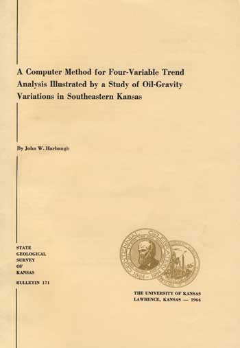
Visualizing the fourth dimension poses a problem. We can, however, represent a fourth variable in three-dimensional space by simply plotting the particular values of the variable at the points where they occur in a three-dimensional coordinate system. In Figure 1, the three axes of a coordinate system are represented by the variables w, x, and y. The fourth variable, z, cannot be graphically represented by an axis, but can be represented by values at different points, the two points, z1 and z2, being shown for illustration's sake.
Figure 1--Method of representing four variables in three-dimensional space. Three variables (w, x, and y) may be represented by values referred to three coordinate axes. Fourth variable (z) can be represented as series of values at specified points in three-dimensional space.
Suppose that we are faced with the problem of representing porosity trends in this block of rock. If the porosity varies in a regular manner, it might be represented by a surface. However, an ordinary surface embedded in three-dimensional space is inadequate because four variables are involved. Consequently we need a four-dimensional surface. A surface of four or more dimensions may be termed a hypersurface, the prefix "hyper" pertaining to above or beyond. Thus, a hypersurface is "above" or "beyond" an ordinary surface in a mathematical sense.
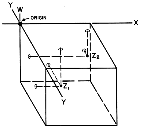
In dealing with data that are irregular ("noisy"), we are commonly faced with the problem of establishing trends. For example, if observations of two variables are plotted on a two-dimensional diagram as a series of points (Fig. 2), the general trend of the points may be represented by a line. The trend line may be fitted by eye, but this is not particularly objective because one person might place the line differently than the next person.
Figure 2--Least-squares fit of line to points. Line has been fitted so that sum of squared deviations (marked with d's) of y with respect to x is minimized.
The problem is to obtain the best fit of the line to the points. The most generally used criterion of best fit is that of least squares. In fitting a line by least squares, the objective is to fit the line so that the sum of the squared deviations of one variable, with respect to the other, is the least possible (Fig. 2). Thus, a least-squares fit is unique because only one position of a line will yield the least possible sum of squared deviations. However, it should be borne in mind that it makes a difference which variable is being minimized. In Figure 2, the trend line has been drawn so that the deviations of y with respect to x have been minimized. The line would have been fitted slightly differently had the objective been to minimize the deviations of x with respect to y. The reason for the difference is that we are not dealing with an ordinary functional relationship in which it makes little difference whether we express y as a function of x, or vice versa. Instead, we are dealing with a correlation in which we seek the best estimate of one variable in terms of the other, either y with respect to x, or x with respect to y.
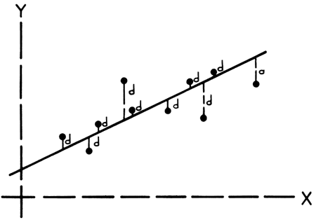
The least-squares criterion is not confined to the fitting of straight lines. Curved lines described by mathematical functions can also be fitted by least squares. Furthermore, the least-squares criterion is applicable to the fitting of planes (Fig. 3), curved surfaces embedded in three-dimensional space, and hypersurfaces.
Figure 3--Least-squares fit of plane to points.
Lines, surfaces, or hypersurfaces that have been fitted by least squares may be described by equations. For example, the equation describing a straight line may be generally written
y = A + Bx
where x and y are variables, and A and B are constants. In this equation, y is the dependent variable, x is the independent variable, A, is the intercept value of the line on the y axis, and the coefficient, B, represents the slope of the line. It is understood that the algebraic sign, plus or minus, is incorporated within these constants. In fitting a straight line by least squares, the problem is to calculate the values of A and B so that the sum of the squared deviations is the least possible. In fitting curved lines, surfaces, or hypersurfaces by least-squares methods, the objective is the same, namely, to obtain the constants of the equations so that the sum of squared deviations is minimized.
The degree of an equation containing a dependent variable and one independent variable is related to the maximum values of the exponents. For example, a second degree equation may be written
y = A + Bx + Cx2
in which x and y are variables and A, B, and C are constants. Similarly, a general equation of the third degree involving one dependent and one independent variable may be written
y = A + Bx + Cx2 + Dx3.
At this point it is convenient to introduce a general classification of equations and their graphic representations according to degree and number of variables. Figure 4 presents a series of equations and their graphs in which degree is listed by column and number of variables by row. For example, in equations of the first degree, two variables yield a straight line, three variables a plane, and four variables a first-degree hypersurface.
The terms within each equation of Figure 4 may be classed according to whether they are linear, quadratic, or cubic. The linear components are those of the first degree, and include the intercept, A, and terms to the first power. The quadratic components include terms containing up to two variables to the first power, or one variable to the second power. Thus, in the equation of the three-variable second-degree surface of the general form (Fig. 4), the linear terms are A + Bx, and the quadratic terms are Dx2 + Exy + Fy2. In Table 1 the terms of the general equations of Figure 4 are classified according to whether they are linear, quadratic, or cubic.
Figure 4--Relationship between number of variables and degree of generalized equations and their geometric equivalents. Degree (first, second, and third) is listed by column and number of variables (two, three, or four) by rows. Variables are denoted by U), x, y, and z, and constants (with algebraic sign implicitly included) by A through T. Two variables are represented geometrically by straight or curved lines, three variables by surfaces, and four variables by hypersurfaces.
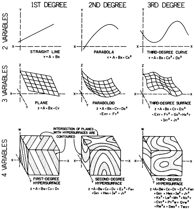
Table 1--Generalized equations classified according to degree and number of variables. The dependent variable has been omitted here.
| Number of variables |
Degree | Descriptive title |
Classification of terms in equation | ||
|---|---|---|---|---|---|
| Linear | Quadratic | Cubic | |||
| 2 | First | Straight line | A + Bx | ||
| Second | Parabola | A + Bx | + Cx2 | ||
| Third | Third-degree | A + Bx | + Cx2 | + Dx3 | |
| 3 | First | Plane | A + Bx + Cy | ||
| Second | Elliptic paraboloid or hyperbolic paraboloid | A + Bx + Cy | + Dx2 + Exy + Fy2 | ||
| Third | Third-degree surface | A + Bx + Cy | + Dx2 + Exy + Fy2 | + Gx3 + Hx2y + Ixy2 + Jy3 | |
| 4 | First | First-degree hypersurface | A +Bw + Cx + Dy | ||
| Second | Second-degree hypersurface | A + Bw + Cx + Dy | + Ex2 + Fwy + Gxy + Hwx + Iw2 + Jy2 | ||
| Third | Third-degree hypersurface | A + Bw + Cx + Dy | + Ex2 + Fwy + Gxy + Hwx + Iw2 + Jy2 | + Kx3 + Lw3 + My3 + Nx2y + Oxw2 + Py2w + Qyw2 + Rw2x + Swx2 + Twxy | |
| Note: Cubic terms with coefficients N through T have been arbitrarily omitted in this study but are listed here for the sake of completeness. | |||||
Four-dimensional surfaces (hypersurfaces) may be visualized. Consider the way in which four variables (w, x, y, and z) may be represented by a coordinate system in three-dimensional space (Fig. 1). Three of the variables (w, x, and y) may be represented as dimensions with respect to three reference axes arranged perpendicular to one another.
The fourth variable, z, may be represented at individual points in space. To these points in space we may fit, by least squares, a plane or curving hypersurface which represents the best estimate of z in terms of the other three variables, w, x, and y. We may visualize such a four-dimensional hypersurface as a series of infinitesimally thin, three-dimensional surfaces nested together. If the hypersurface is intersected by planes, as for example on the top, bottom, and four sides of a block (Fig. 4), the intersections of the hypersurface with the planes of the block may be portrayed by contour lines drawn on the surfaces of the block. A first-degree hypersurface (Fig. 4) might be likened to a series of parallel planes or series of slices, each infinitesimally thin. Higher-degree hypersurfaces may be thought of as formed by an infinite number of nested, curving surfaces rather than planes.
The author gratefully acknowledges the assistance of the following persons: Peter Carah, for help in preparing that part of the computer program for plotting data values; D. F. Merriam, for preparing the oil-gravity data for key punching; Perfecto Mary, for drawing the illustrations; and Mrs. Patricia M. Richmond, for typing the manuscript. In addition, the manuscript was reviewed by R. G. Hetherington, D. F. Merriam, F. W. Preston, E. D. Goebel, and J. M. McNellis, all of whom made valuable suggestions for its revision. However, any errors and/or omissions are the sole responsibility of the author.
The computer program was developed with a grant of computer time from the Computation Center at Stanford University. Part of the grant was made possible through support of the Computation Center by National Science Foundation Grant NSF-GP948.
One of the purposes of this report is to illustrate the use of four-variable hypersurfaces with an example. The example chosen deals with variations in crude oil gravity in southeastern Kansas. Here the problem is to interpret the geologic significance of differences in oil gravity from place to place, and from zone to zone stratigraphically. As an introduction to the problem, the measure of oil gravity is discussed first, followed by a discussion of oil-gravity variations in other regions.
API (American Petroleum Institute standard) gravity is the most widely used measure of the properties of crude oil. API gravity is a function of the density per unit volume, and its relationship to specific gravity is shown by the following formula:
Degrees API = (141.5 / Sp. Gr. at 60°F) -131.5
It should be noted that API gravity increases when specific gravity decreases, and vice versa. Thus, an oil with a high API gravity has a lower specific gravity than an oil with a low API gravity.
Certain other properties of crude oil are generally related to API gravity, including viscosity (which increases with decreasing API gravity) and gross chemical composition. API gravity is a rough measure of the proportions of hydrogen and carbon in crude oil; oils of high API gravity (low specific gravity) are richer in hydrogen than those of lower API gravity. It is believed that the API gravity of an oil is related to the conditions under which the oil originated, including the character of the organic source materials from which it was derived, the chemical and mineralogical composition of the rocks in which it is contained, and the physical conditions, such as temperature and pressure, under which it has "matured" and been stored.
There are a number of references in the literature to oil-gravity gradients of a regional nature, or changes in oil gravity that may be correlated with changes in depth of burial. For example, Barton (1937) presented convincing evidence that the specific gravities of crude oils in the Gulf Coast region generally decrease with depth. When a particular Cenozoic stratigraphic interval is traced downdip, specific gravity of the oil decreases and API gravity increases. Barton suggested that the general decrease in specific gravity with depth reflects the evolutionary processes by which crude oils that were originally napthenic have been gradually converted into paraffinic crudes as an effect of temperature, pressure, and time. He suggested that these changes may be analogous to those in the refining of crude oil, in which the high temperatures and high pressures that prevail for a very short time in the refinery are capable of bringing about drastic changes in the chemical composition of petroleum. Underground, the increases in temperature and pressure that have accompanied deeper burial are much less severe than those encountered in the refinery, but Barton pointed out that the far greater amount of time available geologically may have compensated for less severe temperature and pressure conditions.
Barton's views on Gulf Coast crude oils were challenged by Haeberle (1951) and Bornhauser (1950), who stated that while an increase in API gravity (decrease in specific gravity) can generally be correlated with an increase in depth, the increase in API gravity is not necessarily a simple function of depth of burial, but instead, could be a result of facies changes. As the Cenozoic strata of the Gulf Coastal Region of Texas and Louisiana are traced downdip, they generally exhibit a progressive change from continental facies, to shallow-water marine, and, finally, to deepwater marine facies. In other words, if one wished to ignore changes in depth of burial entirely, one could make an almost equally strong case for control of oil gravities by facies alone. Thus, the deep-water marine sediments, consisting mostly of shale, yield oil of highest API gravity, whereas near-shore sediments, which contain larger proportions of sand, yield oil that is lower in API gravity. Due to the imbricate, wedge-like aspect of the strata of the Gulf Coast, a well tends to pass downward from near-shore sediments to deeper-water sediments. Thus, the oil-gravity changes encountered in different reservoirs in a single well, or the changes of oil gravity in a series of wells in which a given stratigraphic horizon is followed downdip, both tend to exhibit changes in oil gravity that could be interpreted as facies-controlled or depth-controlled. Obviously, in the Gulf Coast we are dealing with a problem in which correlations are simple enough to establish, but cause and effect relationships are more obscure.
Hunt (1953) studied the variations of API gravity in crude oils in Wyoming, where the geology is more complicated than in the Gulf Coast. He came to two principal conclusions:
(1) There is a strong correlation of API gravity and other measures of the composition of crude oils with environment of deposition of the reservoir rocks in which the oils occur. Relatively low API gravity oils are associated with Paleozoic sediments, formed under quiet, stable conditions of moderate to high salinity, in which carbonates and sulfates were abundant. High API gravity oils tend to be associated with Mesozoic sediments, formed under conditions of moderate tectonic activity, in which dark shales predominate, with discontinuous sandstones and a few thin beds of limestone. Thus, environment of deposition, including the character of organic source materials, seems to be the most important factor affecting API gravity in Wyoming. (2) There is, however, a relationship between depth of burial and API gravity in Wyoming, provided that the oils are separated into two major groups, Paleozoic and Mesozoic. Hunt found that there is an overall increase in API gravity with depth of occurrence of oils in Paleozoic rocks and similarly with oils in Mesozoic rocks. However, the deepest Paleozoic oils are of a lower API gravity than are the shallowest Mesozoic oils. Hunt's (1953, p. 1,865) plot of API gravity versus depth of oil in the Paleozoic Tensleep Formation suggests that there is an almost linear increase in API gravity with depth. Hunt concluded that depth of burial cannot be ignored, but that it is of secondary importance.
Hitchon et al. (1961) showed that there is an apparent progressive increase in API gravity downdip east of the Canadian Rockies in Mississippian, Pennsylvanian, Permian, Triassic, Jurassic, and some Cretaceous and Devonian strata. However, there is no regular increase in API gravity downdip in certain other Devonian and Cretaceous strata in the region. The cause of geographic variations in API gravity in western Canada is poorly understood. Hitchon et al. (1961, p. 296) suggest that in some stratigraphic units, high API gravities tend to occur in tectonic basin areas and low API gravities in shelf areas.
Smith (1963) pointed out that the specific gravity of oil produced from the Green River oil shales in Colorado decreases systematically with increasing depth of burial. Smith fitted by least squares a series of second-degree (parabolic) curves relating specific gravity to depth in individual bore holes. He stated that the decrease in specific gravity is associated with a progressive decrease in oxygen content with depth, which in turn may have resulted from loss of carboxyl groups from organic molecules due to increase of heat and pressure with increasing depth.
A research committee of the Tulsa Geological Society, consisting of Neumann et al. (1947), conducted a study of variations in crude oil in southeastern Kansas and adjacent northeastern Oklahoma. They concluded that the environment of deposition and the original character of the oil's organic source material probably determined the kind of oil in each pool. For example, they found that the oil in the "Bartlesville sand" of Osage County, Oklahoma, could be divided into six classes on the basis of distillation fractions. Pools in the "Bartlesville sand" containing particular classes of oil have distinct geographical groupings. Neumann's committee suggested that the area in which a particular class of oil occurs reflects a particular set of depositional conditions that prevailed in that area. They found little evidence that the oil migrated over appreciable distances, and they concluded that the oil formed mostly from organic materials deposited close to the places where the oil now occurs.
Recent findings by Baker (1962) support the conclusions of Neumann's committee. Baker compared the distribution of traces of hydocarbons in nonreservoir facies close to the shoestring sand reservoirs in the Pennsylvanian Cherokee Group ("Bartlesville sand" or "Burbank sand"), in the Thrall (Thrall-Aagard) field in Greenwood County, Kansas, and in the Burbank field in Osage County, Oklahoma. Baker found that the proportions of hydrocarbons (expressed as the ratio of saturate hydrocarbons to aromatic hydrocarbons) in the nonreservoir facies tend to parallel those of the crude oil produced in the adjacent oil fields. He found that traces of hydrocarbons extracted from the nonreservoir facies encountered in a core in the Burbank field have significantly higher saturate to aromatic ratios than hydrocarbons from nonreservoir facies close to the Thrall field. Burbank crude also has a higher saturate to aromatic ratio than Thrall crude. It is presumed that differences in the crude oils reflect differences in trace hydrocarbons extracted from associated, nonreservoir rocks. Consequently, both trace hydrocarbons and crude oil appear to have a similar source within a given locality.
Oil-gravity data used in this study were taken from a report by Everett and Weinaug (1955) and include API gravity measured at 60°F, well location, depth to producing zone, and name of producing zone. The oil-gravity data were studied in a rectangular area (Fig. 5) about 65 by 70 miles in dimension, which embraces Chautauqua, Cowley, and Elk counties, and parts of Greenwood, Butler, Woodson, Wilson, and Montgomery counties. The location of wells for which API gravity was determined is shown in Figure 5 and the wells are numbered by Everett and Weinaug (1955, p. 211-221) as follows: 8, 13 to 22, 30 to 35, 41 to 44, 55 to 93, 95 to 104, 107 to 137, 145 to 222, 224, 227 to 230, 232, 234 to 250, 386 to 397, 400, 404 to 406, 411 to 419, 421 to 426, 428, 444 to 447, 449 to 453. Data on wells listed by Everett and Weinaug that lie outside the area of this study were not used. A total of 244 API gravity values were used. The geographic distribution of wells yielding oil-gravity data is somewhat uneven, due largely to the uneven distribution of oil fields within the area (Fig. 6). In addition, the distribution of the gravity values according to well depth is also somewhat uneven. Accordingly, the data points used in this study are not randomly distributed in space.
Figure 5--Map of part of southeastern Kansas showing location of oil wells yielding oil-gravity data used in this study.
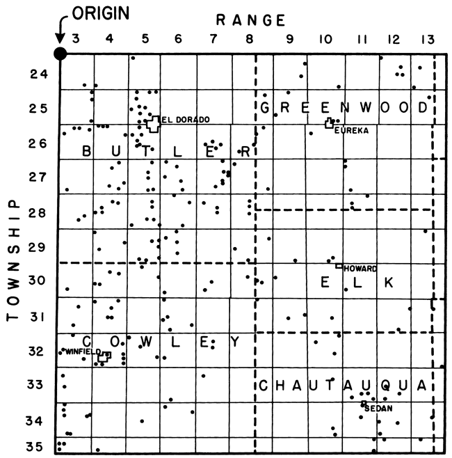
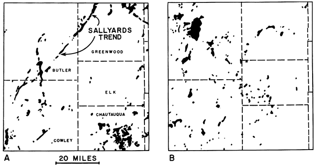
Figure 6--Maps showing outlines of oil fields in part of southeastern Kansas (modified froni Goebel, Hilpman, Beene, and Noever, Pl. 1, 1962). (A) Oil fields in which oil occurs principally in lenticular sands. or in shoestring sands, and in which accumulation of oil is mainly stratigraphically controlled. (B) Oil fields in which oil occurs principally in carbonate reservoir rocks and in which structural control of oil accumulation is important.
Oil is produced from various stratigraphic zones in the area of this study in southeastern Kansas (Table 2). The names of some of the zones are local drillers' terms that are not official geological names. Jewett (1954, p. 76-90) provides glossary of names of oil-producing zones in eastern Kansas, and the approximate stratigraphic position of the zones is given in a columnar chart by Jewett (1959).
Table 2--Local terms and stratigraphic position of oil-producing zones in area of study.
| Oil-producing zone | Group | Stage | System |
|---|---|---|---|
| Admire | Admire | Gearyan | Permian |
| Topeka Limestone "Peacock sand" |
Shawnee | Virgilian | Pennsylvanian |
| "Hoover sand" | |||
| "Stalnaker sand" | Douglas | ||
| Lansing | Lansing | Missourian | |
| "Layton sand" | Kansas City | ||
| "Kansas City lime" | |||
| "Wayside sand" | Marmaton | Desmoinesian | |
| "Peru sand" | |||
| "Cattleman sand" "Bartlesville sand"* "Burgess sand" |
Cherokee | ||
| "Mississippi chat" | Meramecian | Mississippian | |
| "Mississippi lime" | |||
| Viola Limestone | Middle Ordovician | Ordovician | |
| "Simpson sand" | Simpson | ||
| Arbuckle Limestone | Arbuckle | Lower Ordovician | |
| *Note: "Bartlesville sand" is a general name given certain lenticular oil-producing sands that vary slightly in age and stratigraphic position from place to place. | |||
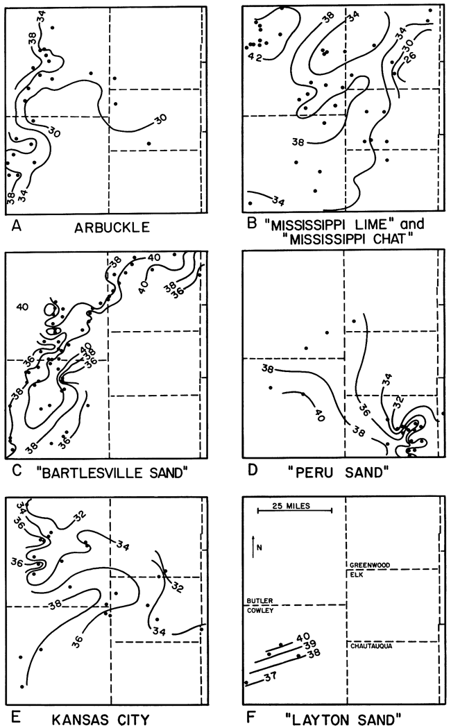
The distribution of API gravities in six stratigraphic zones in part of southeastern Kansas is shown on maps in Figure 7. The stratigraphic position of each zone is given in Table 2. The maps show that (1) in detail, areal variations in API gravities are erratic, but (2) that broad scale trends are present. API gravities of oils in the Arbuckle Limestone and Kansas City Group (Fig. 7A, 7E) generally increase toward the west, and API gravities in the "Mississippi lime" and "Mississippi chat" and "Layton sand" (Fig. 7B, 7D, 7F) generally increase toward the northwest. API gravities in the "Bartlesville sand" (Fig. 7C) are more erratic, and gross changes across the area are not apparent.
Figure 7--Contour maps showing variations of API gravity in different stratigraphic zones in southeastern Kansas. (Dots mark locations of oil wells.) (See Fig. 5 for location of township and range.)
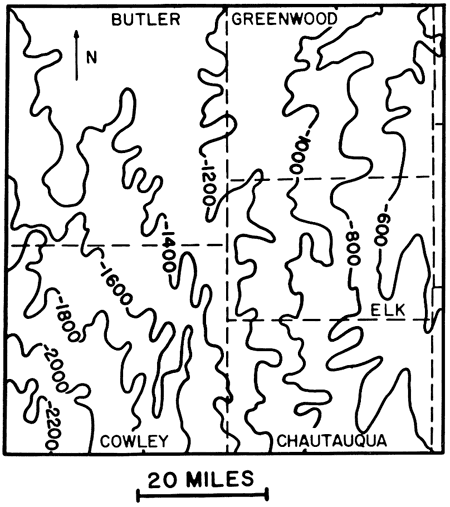
Considering the oil-producing zones in general, there is a downdip increase in API gravity, the regional structure being a west-dipping homocline (Fig. 8).
Figure 8--Structure contour map on top of Mississippian rocks in part of southeastern Kansas (after Merriam, 1960). Contour values in feet. (See Fig. 5 for location of township and range.)
Thus, the question arises, is the increase in API gravity toward the west due to increasing depth, or is it related to geographic position?
Some other aspects of the geographic distribution of API gravities are worth noting. The distribution of API gravities in the "Bartlesville sand" (Fig. 7C) appears to parallel the "Sallyards shoestring" trend (Fig. 6A). Bass et al. (1937) have interpreted this trend, as well as other shoestring sand deposits, to be ancient offshore bars formed at the shifting margin of a Pennsylvanian sea. Perhaps variations in environmental conditions during Pennsylvanian time are responsible for much of the variation in oil gravities in the "Bartlesville sand."
Within the area, the "Bartlesville sand" has the highest average API gravity with values ranging from a little less than 36° API to greater than 40° API (Fig. 7C). However, the range of gravity variations is greater in oil obtained from the "Mississippi lime" and the "Mississippi chat" (Fig. 7B). Some geologists have speculated that oil in the "Mississippi chat" and "Mississippi lime" has been derived from shale in the overlying Cherokee Group, which contains the "Bartlesville sand" and other oil-producing sands. However, the contrast of API gravities in the "Mississippi lime" and "chat" with those in the "Bartlesville" suggests that the oils may be of differing sources.
First-, second-, and abbreviated third-degree trend hypersurfaces have been fitted to oil-gravity data in southeastern Kansas, and the results are appraised statistically and geologically below. A glossary of statistical terms used but not explained otherwise is provided later in this report.
Frequency distribution of original oil-gravity data and of first-, second-, and third-degree trend and residual (deviation) values is shown in a series of histograms in Figure 9. The original data (Fig. 9A) are somewhat skewed so that the mean is displaced to the left, or low side, of the median. The distribution of natural logarithms of the original data (Fig. 9B) is more symmetrical, although logarithmic transformations of original data were not deemed necessary in this study.
Figure 9--Histograms of frequency distributions of original API gravity data, logarithmically transformed data, and trend and residual values. Numbers beneath histograms refer to midpoint values within each frequency class.
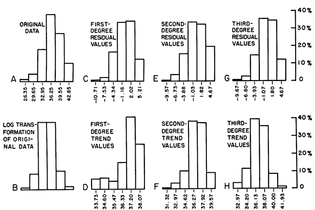
The characteristics of the frequency distributions of trend and residual values are important in analysis of variance to determine confidence levels because more or less symmetric frequency distributions of trend and residual values are desirable. The histograms (Fig. 9) of residual values (Fig. 9C, E, G) reveal moderate skewness, partly reflecting the skewness of the original data. The distributions of the trend values (Fig. 9D, F, H) are also somewhat skewed. However, it is concluded that the frequency distributions are not sufficiently skewed to invalidate use of analysis of variance.
Analysis of variance may be used to determine the statistical significance of trend surfaces (Dawson and Whitten, 1962, p. 8; Allen and Krumbein, 1962, p. 522-523). In this study, the objective has been to determine the degree of confidence for each component of the hypersurfaces, or, in other words, to determine whether the linear, quadratic, and cubic components are statistically significant or could be due to chance alone. The degree of confidence is spoken of as the "confidence level," and may be expressed in percent. On this basis, absolute certainty is 100 percent, and absolute uncertainty is 0 percent. A confidence level of 99 percent for a particular component would indicate 99 percent certainty that the component represents a real effect and not chance.
Table 3 includes the basic data for calculation of confidence levels by analysis of variance. The data include (a) sum of squares that are apportioned among the linear, quadratic, and abbreviated cubic components, respectively, (b) sums of squares associated with the deviations or residuals, and (c) number of degrees of freedom associated with the components and the deviations. These data, in turn, permit (d) calculation of the mean square of the components and deviations and (e) calculation of Snedecor's F. Finally, (f) the confidence level in percent is obtained by reference to tables of F (Snedecor, 1956, p. 246-249).
Table 3--Analysis of variance of oil-gravity trend hypersurface data.
| Source | Sum of squares |
Degrees of freedom |
Mean square |
Snedecor's F |
Confidence level |
|---|---|---|---|---|---|
| Total, 244 data points | 333,019.5 | 243 | |||
| Due to linear component | 330,624.2 | 3 | 110,208.1 | 10,054.0 | 99.9 + % |
| Deviations from linear | 2,395.3 | 240 | 10.0 | ||
| Due to quadratic component | 252.6 | 6 | 42.1 | 4.6 | 99.9 + % |
| Deviations from quadratic | 2,142.7 | 234 | 9.1 | ||
| Due to abbreviated cubic component | 189.1 | 3 | 63.0 | 7.5 | 99.9 + % |
| Deviations from abbreviated cubic | 1,953.6 | 231 | 8.5 |
The number of degrees of freedom is established in reference to (1) the number of degrees of freedom associated with the total number of data points (n - 1), and (2) number of terms containing variables in the equation belonging to each component. Thus, there are three degrees of freedom associated with the three linear terms Bw, Cx, and Dy; six degrees of freedom with the six quadratic terms Ex2, Fwy, Gxy, Hws, Iw2, and Jy2; and three with the cubic terms Kx3, Lw3, and My3. The number of degrees of freedom at each level is obtained by successively subtracting the degrees of freedom associated with each component from the degrees of freedom associated with the data points.
The confidence levels associated with the three trend components of the oil-gravity data are extremely high, all being in excess of 99.9 percent. It is concluded that the effect associated with each component is real and not fortuitous.
The percent of total sum of squares is a measure of how closely the hypersurfaces (Table 4) fit the observed data and is calculated according to an equation given in Appendix A. A percent of total sum of squares of 100 percent would represent a perfect fit of the observed data. There is a general relationship between the confidence level associated with a component, and the percent of total sum of squares associated with that component.
Table 4--Percent of total sum of squares represented by hypersurfaces fitted to oil-gravity data.
| Linear surface | 32.0% |
| Linear + Quadratic surface | 49.7% |
| Linear + Quadratic + Abbreviated Cubic surface | 63.0% |
If there is a marked increase in percent of total sum of squares when a new component is included, a high confidence level is generally associated with that component (Table 3) and vice versa.
Spatially weighted averages (Table 5) of API gravity have been calculated for each hypersurface by the method described in Appendix A. The resulting averages are close to the arithmetic mean. Little advantage is gained in this case by calculation of spatially weighted averages.
Table 5--Averages (API degrees) of oil-gravity values in southeastern Kansas.
| Arithmetic mean | 36.79° |
| Average value within first-degree hypersurface | 35.87° |
| Average value within second-degree hypersurface | 36.33° |
| Average value within third-degree hypersurface | 36.96° |
Trend hypersurfaces fitted to API gravity data are shown in block diagrams (Fig. 10) in which contour lines portray the intersections of sides of the blocks with the hypersurfaces.
Figure 10--Hypersurfaces (A-C) fitted to API gravity data with respect to depth below surface and geographic location. Block D shows generalized geologic structure. Equations of hypersurfaces are listed.
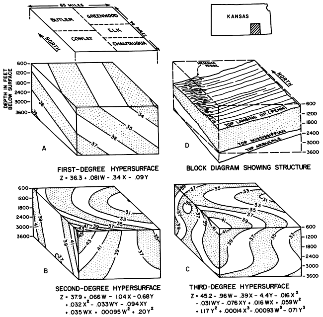
The first-degree hypersurface (Fig. 10A) represents the observed data moderately well, accounting for about 32 percent of the total sum of the squares (Table 4). The confidence level (Table 3) is in excess of 99.9 percent, signifying that the first-degree trend hypersurface represents a real effect and cannot be due to chance alone.
The first-degree hypersurface may be likened to an east-southeast-dipping homocline, reflecting trends in the original data, namely that (1) at a given depth there is a general increase in API gravity toward the west-northwest, and (2) at any particular locality, there is a general increase in API gravity with depth. The first-degree hypersurface makes clear that differences in API gravity are not segregated in any uniform manner according to depth or to stratigraphic zones because the planes within the first-degree hypersurface dip toward the east, whereas the strata dip generally toward the west (Fig. 8; 10D).
The second-degree hypersurface (Fig. 10B) reveals trends that differ considerably from the first-degree hypersurface. The second-degree hypersurface might be likened to a complex syncline that plunges toward the east-southeast on one side, but the direction of plunge and shape of the hypersurface are gradually reversed, as is revealed by contours on the south-facing or front side of the block. We are dealing with a series of complex, nested surfaces within the hypersurface, and the shape of any particular surface, as for example the 37° API surface, is that of a saddle-shaped hyperbolic paraboloid. The second-degree hypersurface represents a percent of the total sum of the squares of about 50 percent (Table 4), and the confidence level associated with the quadratic component is in excess of 99.9 percent (Table 3).
Interpretation of the geologic significance of the second-degree hypersurface is somewhat difficult because the surface is more complex than the first-degree hypersurface. The increased complexity reflects the improved fit of the hypersurface and emphasizes that oil-gravity values vary in a complex manner within the area.
Although the third-degree hypersurface (Fig. 10C) is still more complex than the second-degree hypersurface, there are marked similarities between the two. Surfaces within the third-degree hypersurface may be likened to an eastward-plunging, complex syncline that gradually becomes a saddle-shaped structure. The percent of total sum of squares represented by the third-degree surface is about 63 percent (Table 4), and the contribution of the abbreviated cubic component (the cubic cross product terms have been omitted) is real, since a confidence level of more than 99.9 percent is associated with it (Table 3).
The third-degree hypersurface also reflects the increase in API gravities toward the west, but it suggests that the increase is by no means a simple increase in that direction. Furthermore, it appears to bear a relationship to the low API gravities in the Arbuckle, or lowest oil-producing zone, as indicated by the westward deflection of the contour lines near the bottom of the south-facing side of the block (Fig. 10C).
The generalized spatial distribution of positive and negative second-degree residual oil-gravity values is shown in a series of "slice maps" (Fig. 11A), and distribution of positive residuals is shown in a block diagram (Fig. 11B). The residual values were obtained by subtracting trend values from observed values. The spatial distributions of first- and third-degree residual values are almost the same as the second-degree residuals and are not shown here. Considering the positive residuals within the block extending from 1200 to 3600 feet (well depth), there are three main places where positive values congregate: (1) in the extreme southeast corner of the block, (2) in the extreme northwest corner of the block, and (3) in a broad and very irregular zone that extends from northeast to southwest across the block. The negative residuals are aggregated between the positive residuals.
The clusters of residual values reflect variations in the original data. The positive cluster that trends northeast-southwest across the block partly reflects high API values in the "Bartlesville sand" (Fig. 7C) in the Sallyards trend (Fig. 6A). However, it is interesting to note that this cluster also includes oil-producing zones that lie both above and below the "Bartlesville sand." This is important because it suggests that factors responsible for relatively high API gravities in this cluster are common to various stratigraphic zones and not just the "Bartlesville" alone.
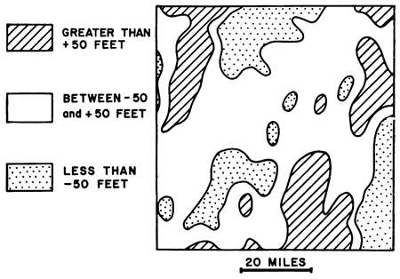
An interesting comparison can be made between the areal distribution of structural residual values and API oil-gravity residual values. Figure 12 shows the clusters of structural residual highs and lows produced when a second-degree, three-variable trend surface is subtracted from the structure on top of Mississippian rocks in this same part of southeastern Kansas (Fig. 8). There are several structural residual lows which trend in a northeast-southwest direction across the area. This northeast-southwest trend coincides more or less with the cluster of positive oil-gravity residual values (Fig. 11). In addition, there are residual structural lows toward the southeast and northwest corners of the area, roughly in the same places where the other two API gravity residual highs occur. Structural highs of the Nemaha ridge (Figs. 8; 10D) seem associated with oil-gravity lows, but this may be due in presence of relatively low-gravity Arbuckle fields (Figs. 6B; 7A) in that part of the area. The coincidence between residual oil-gravity highs and residual structural lows may not be fortuitous, and perhaps similar relationships occur in other areas.
Figure 11--Distribution of second-degree residual values of API gravity in three-dimensional space. (A) Series of four slice maps, each representing 600-foot depth interval, showing clustering of residual values. (B) Block diagram showing clustering of positive residual values.
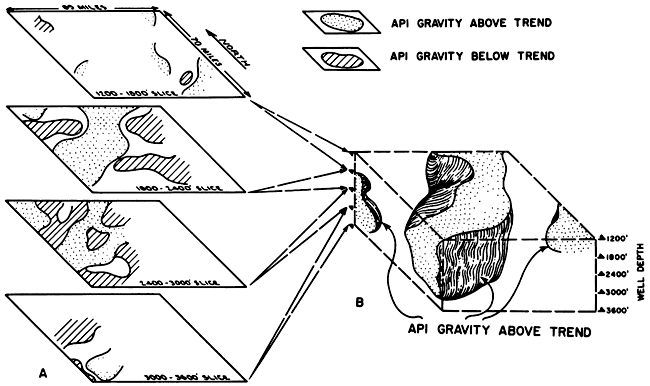
Figure 12--Simplified contour map of residual values obtained by subtracting second-degree trend surface fitted to structure on top of Mississippian rocks (Fig. 8) in area of study.
The tendency for oil-gravity residual values from different stratigraphic zones to be aggregated into the same clusters may reflect long-persisting ancient geographic and environmental conditions. For example, during part of Pennsylvanian time, limestone marine banks that formed in southeastern Kansas (Harbaugh, 1960, p. 229-232) tended to be stacked one upon another in the same general localities, in spite of occurring in different stratigraphic units. It is presumed that the marine banks were a localized response to environmental conditions that included water depths, waves, currents, and sources of terrestrially derived sediment. These environmental conditions, in turn, probably reflected large-scale ancient geographic conditions, such as the configuration of land and sea. It is speculated that oil-gravity residual clusters in southeastern Kansas may also partly reflect ancient geographic and environmental features that may have persisted during much of the Paleozoic Era. For example, the ancient geography may have influenced the distribution of marine organisms, including the phytoplankton, and in turn, influenced the characteristics of crude oil formed from organic material incorporated into the sediments. However, these suggestions are tentative and additional study is needed before final conclusions are drawn.
1. There is broad correlation between well depth and API gravity; API gravities tend to increase with depth.
2. Factors other than depth appear to have a strong influence, however. These factors might generally be classed as depositional environment factors.
3. The first-degree hypersurface (Fig. 10A) makes clear that oil-gravity variations are not controlled by progressive changes between stratigraphic zones, because planes within the first-degree hypersurface dip opposite to the strata (Fig. 10D).
4. Similar environmental factors may have influenced oil gravities in different stratigraphic zones in the same general localities. This is suggested by aggregation of residual values in distinct clusters in three-dimensional space.
5. The tendency for residual values to be clustered suggests that depositional conditions affecting oil gravities in a given locality may have remained more or less the same during much of the Paleozoic. If this is the case, dual clusters could represent responses to long-persisting ancient geographic features, such as shore lines, sediment source areas, and organism communities, which affected the depositional environment at any particular place for long intervals of time.
6. It is suggested that both depth of burial and depositional environment have influenced oil-gravity values. Of the two, perhaps depositional environmental factors are the most important.
Analysis of variance. A technique in which the variation within a set of data is separated into different components, permitting differences between and within components to be compared. Ordinarily, the estimate of variance is:
V = σ2 = [Σ (x - ![]() )2] / (n-1)
)2] / (n-1)
where V = variance,
n = number of data values,
x = observed data values,
![]() = arithmetic mean,
= arithmetic mean,
σ = standard deviation.
However, in this study, analysis of variance was used to determine the significance of trend hypersurfaces, and mean square values were used instead of variance estimates.
Degrees of freedom. Pertains to the number of opportunities in which variation may occur. For example. a set of data containing 10 data values has nine degrees of freedom. Similarly, a set with one data value contains zero degrees of freedom, because no variation is possible.
Snedecor's F. The ratio of two variances, or the ratio of two mean squares.
Frequency distribution. Pertains to the manner in which a set of data values are distributed according to frequency of occurrence.
Logarithmic transformation. Involves use of logarithms of data values rather than the raw data values themselves.
Mean square. Refers to the sum of squares divided by the number of degrees of freedom:
mean square = sum of squares / degrees of freedom
Residual values (deviations). Obtained by subtracting trend values from observed values.
Skewness. Pertains to the degree of asymmetry in a frequency distribution.
Sum of squares. The sum of squared values.
Trend values. Values estimated on the basis of a trend line or surface. For example, if a trend line is fitted to points on an X-Y diagram, for each value of Y there is a corresponding estimate of X.
Allen, Percival, and Krumbein, W. C., 1962, Secondary trend components in the top Ashdown Pebble bed: A case history: Jour. Geol., v. 70, no. 5, p. 507-538.
Baker, D. R., 1962, Organic geochemistry of Cherokee Group in southeastern Kansas and northeastern Oklahoma: Am. Assoc. Petroleum Geologists Bull., v. 46, no. 7, p. 1621-1642.
Barton, D. C., 1937, Evolution of Gulf Coast crude oil: Am. Assoc. Petroleum Geologists Bull., v. 21, no. 7, p. 914-946.
Bass, N. W., Leatherock, Constance, Dillard, W. R., and Kennedy, L. E., 1937, Origin and distribution of Bartlesville and Burbank shoestring oil sands in parts of Oklahoma and Kansas: Am. Assoc. Petroleum Geologists Bull., v. 21, no. 1, p. 30-66.
Bornhauser, Max, 1950, Oil and gas accumulation controlled by sedimentary facies in Eocene Wilcox to Cockfield Formations, Louisiana Gulf Coast: Am. Assoc. Petroleum Geologists Bull., v. 34, no. 9, p. 1887-1896.
Dawson, K. R., and Whitten, E. H. T., 1962, The quantitative mineralogical composition and variation of the Lacorne, La Motte, and Preissac granitic complex, Quebec, Canada: Jour. Petrology, v. 3, p. 1-37.
Everett, J. P., and Weinaug, C. P., 1955, Physical properties of eastern Kansas crude oils: Kansas Geol. Survey, Bull. 114, pt. 7, p. 195-221.
Goebel, E. D., Hilpman, P. L., Beene, D. L., and Noever, R. J., 1962, Oil and gas developments in Kansas during 1961: Kansas Geol. Survey, Bull. 160, p. 1-231.
Haeberle, F. R., 1951, Relationship of hydrocarbon gravities to facies in Gulf Coast: Am. Assoc. Petroleum Geologists Bull., v. 35, no. 10, p. 2,238-2,248.
Harbaugh, J. W., 1960, Petrology of marine bank limestones of Lansing Group (Pennsylvanian), southeast Kansas: Kansas Geol. Survey, Bull. 142, pt. 5, p. 189-234. [available online]
Harbaugh, J. W., 1963, BALGOL program for trend-surface mapping using an IBM 7090 computer: Kansas Geol. Survey, Special Dist. Pub. 3, 17 p.
Hitchon, Brian, Round, G. F., Charles, M. E., and Hodgson, G. W., 1961, Effect of regional variations of crude oil and reservoir characteristics on in situ combustion and miscible-phase recovery of oil in Western Canada: Am. Assoc. Petroleum Geologists Bull., v. 45, no. 3, p. 281-314.
Hunt, J. M., 1953, Composition of crude oil and its relation to stratigraphy in Wyoming: Am. Assoc. Petroleum Geologists Bull., v. 37, no. 8, p. 1,837-1,872.
Jewett, J. M., 1954, Oil and gas in eastern Kansas: Kansas Geol. Survey, Bull. 104, p. 1-397.
Jewett, J. M., 1959, Graphic column and classification of rocks in Kansas: Kansas Geol. Survey, chart.
Krumbein, W. C., 1956, Regional and local components in facies maps: Am. Assoc. Petroleum Geologists Bull., v. 40, no. 8, p. 2,163-2,194.
Krumbein, W. C., 1959, Trend surface analysis of contour-type maps with irregular control-point spacing: Jour. Geophysical Research, v. 64, no. 7, p. 823-834.
Merriam, D. F., 1960, Preliminary regional structural contour map on top of Mississippian rocks in Kansas: Kansas Geol. Survey, Oil and Gas Invest. 22, map.
Neumann, L. M., Bass, N. W., Ginter, R. L., Mauney, S. F., Newman, T. F., Ryniker, Charles, and Smith, H. M., 1947, Relationship of crude oils and stratigraphy in parts of Oklahoma and Kansas: Am. Assoc. Petroleum Geologists Bull., v. 31, no. 1, p. 92-148.
Peikert, E. W., 1962, Three-dimensional specific-gravity variation in the Glen Alpine stock, Sierra Nevada, California: Bull. Geol. Soc. America, v. 73, no. 11, p. 1,437-1,448.
Peikert, E. W., 1963, IBM 709 program for least squares analysis of three-dimensional geological and geophysical observations: Tech. Report No. 4, Contract Nonr-1228 (26), Office of Naval Research, Geography Branch.
Smith, J. W., 1963, Stratigraphic change in organic composition demonstrated by oil specific gravity-depth correlation in Tertiary Green River oil shales, Colorado: Am. Assoc. Petroleum Geologists Bull., v. 47, no. 5, p. 804-813.
Snedecor, G. W., 1956, Statistical methods: Iowa State College Press, p. 534.
Whitten, E. H. T., 1962, A new method for determination of average composition of a granite massif: Geochimica et Cosmochimica Acta, v. 26, p. 545-560.
Next Page--Appendices and Code
Kansas Geological Survey, Oil-gravity Variations
Placed on web Jan. 25, 2012; originally published in 1964.
Comments to webadmin@kgs.ku.edu
The URL for this page is http://www.kgs.ku.edu/Publications/Bulletins/171/index.html