 |
|
Kansas Geological Survey Open-file Report 2003-30 |
Model Architecture
To keep model size manageable, yet accurately reflect the fine scale vertical and horizontal heterogeneity over the entire Panoma Field in Kansas, the Council Grove was subdivided during the lithofacies, porosity and permeability modeling phase. The Panoma was divided horizontally into seven genetically related stratigraphic units, A1 (Funston) through C (Neva). Each is a cycle that has a non-marine interval underlain by a marine interval (e.g.: A1SH and A1LM). The seven permeability models will be joined and uspcaled in the later reservoir simulation phase.
Proportional layering method results in layers proportional to mean thickness of the interval being layered. Number of non-marine interval layers equals the number of feet in the thickness mean. Number of marine interval layers equals mean thickness in feet plus one standard deviation. Marine and non-marine intervals were carried through each model resulting in 12 “dummy” layers in each.
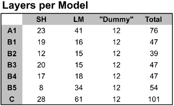 |
Cell size for the modeling is 1000 X 1000 feet, resulting in an average of 8.6 million cells per 5,200 square mile model. The largest model has15 million, the C cycle, and the smallest has 5.7 million, the B2 cycle. Approximately 11 million cells are in the model highlighted in this poster, the A1 cycle. |
Defining the Structural Framework for Panoma
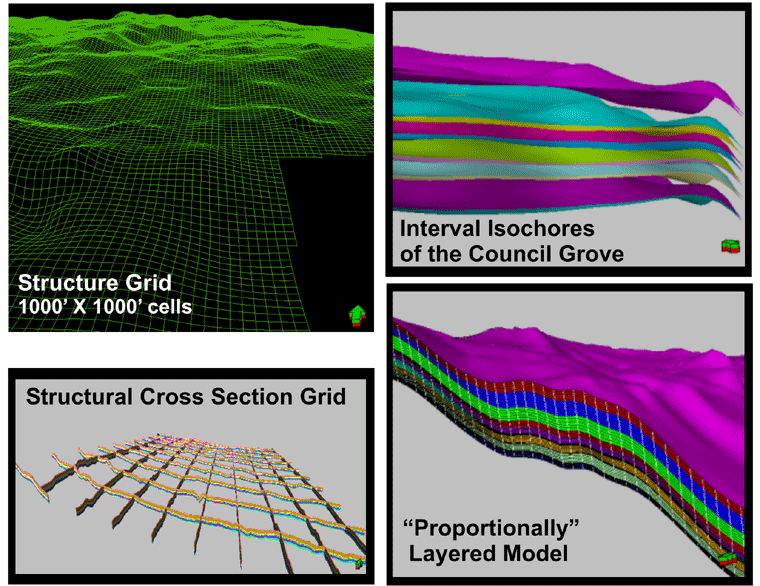
- Create a "skeleton grid" defining the cell size for the model. For Panoma a grid cell size of 1,000' x 1,000' was used to maximize the number of wells for the model to honor exactly. Populating a cell with more than one well results in an "averaging" of those two (or more) data points.
- Construct a top horizon using the Council Grove Group top (A1_SH). Then create isochores for each of the subjacent zones and hang those isochores from the top horizon.
- Fill the newly created horizons with layers thus defining the cell thickness. The Panoma model used "proportional" layering keeping the same number of layers through a given interval regardless of thickness variations. For non-marine shale intervals layer thickness was defined by the average thickness in the zones, and for limestones layer thickness was defined by the average zone thickness PLUS one standard deviation.
- Create general intersection cross-sections to QC structural framework.
|
|
|
e-mail : webadmin@kgs.ku.edu
Last updated May 2003
http://www.kgs.ku.edu/PRS/publication/2003/ofr2003-30/P3-02.html