Kansas Geological Survey, Open-file Report 2007-4
by
David P. Young, Donald O. Whittemore, and Blake B. Wilson
with Appendix by James J. Butler, Jr.
on re-analysis of 1968 pumping-test data for municipal wells of Phillipsburg
KGS Open File Report 2007-4
Prepared for the
Kansas Department of Agriculture,
Division of Water Resources
October 2006
The Division of Water Resources (DWR) of the Kansas Department of Agriculture contracted with the Kansas Geological Survey (KGS) to prepare a bedrock surface coverage and specific capacity data set for the alluvial valleys of the upper forks of the Solomon River basin for use in numerical modeling of ground-water flow in northwest Kansas. The purpose of the ground-water model is to understand the nature of interactions between the river and the alluvial aquifer and between the Ogallala-High Plains and alluvial aquifers, and the effect of ground-water pumpage for management of the water resources in the Ogallala-High Plains aquifer and the Solomon River basin.
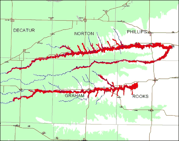
The specific area of study included the spatial extent of the alluvial aquifers of the upper North Fork and the upper South Fork of the Solomon River and its major tributaries down to Kirwin and Webster reservoirs, respectively (Figure 1). The KGS also used depth-to-bedrock data for the area between the alluvial aquifers where the upper Solomon River valleys overlie the Ogallala-High Plains aquifer in order to make the bedrock surface coverage generated for this study consistent with the bedrock surface coverage for the Ogallala-High Plains aquifer region. In addition, we used selected logs with depth-to-bedrock information in the area just outside the extent of the alluvial aquifers of the upper Solomon River basin where the Ogallala-High Plains aquifer is not present. Thus, the overall area where we considered data for the bedrock surface coverage was larger than the specific location of the alluvial aquifer extent.
We assembled a data set for the depth to bedrock below land surface using the water-well logs filed by well drillers in Kansas (WWC-5 records) and test-hole information in KGS publications. We assessed the character of each well log to determine its value for use in preparing a bedrock surface coverage; those records determined to be of questionable value for the purposes of this study were not incorporated in the data set. We constructed a data set that included the depths-to-bedrock along with location and other associated information. These data were used along with point values for the bedrock surface underlying the Ogallala-High Plains aquifer that Macfarlane and Wilson (2006) recently generated. The points in the Macfarlane and Wilson (2006) data set were evaluated in terms of their appropriateness for the bedrock surface that we generated for this study. A few of the prior points were disregarded based on this assessment.
The data set for the bedrock surface is included in spreadsheet format in Appendix A [Microsoft Excel file]. GIS procedures used in the production of the surface are in Appendix B. For each data point, the primary data include Public Land Survey System (PLSS) location (the quarter section designations are in the legal format and are ordered from smallest to largest), source, surface elevation (for published logs with elevations listed), and depth to bedrock below land surface. We determined latitude/longitude locations with the KGS LEO program, using the PLSS locations as input. Surface elevations (for logs without published elevations) were assigned from the National Elevation Dataset (NED; U.S. Geological Survey, 1999). We calculated bedrock surface elevations by subtracting the depth-to-bedrock elevations from the surface elevations. All elevations are in feet.
Data points in the mapped alluvium extent (Figure 1) are flagged in the 'Alluvium' field/column of the data set. New data points are differentiated from existing points from Macfarlane and Wilson (2006) in the 'Source' field/column. New data begin with the suffix 'SOL' and existing data begin with 'OGL'.
Figure 1. Delineation of the study area (shaded in red) in northwest Kansas that includes the extent of the alluvial aquifers of the upper North Fork of the Solomon River down to Kirwin Reservoir and the upper South Fork of the Solomon River down to Webster Reservoir. The extent of the Ogallala-High Plains aquifer is shaded in light green.
There is uncertainty in the bedrock surface due mainly to the non-uniform data density of the points distribution. Further, the elevation of the bedrock surface varies greatly over short distances and reflects whether a well or test-hole log was located in the bottom of a channel cut into the bedrock or on the channel side or underlying a terrace deposit. For example, six test holes drilled in the SE/4 of the SW/4 of Sec. 26, T. 04 S., R. 18 W. (Leonard, 1952) have bedrock elevation differences greater than 30 ft. Of those test holes, the greatest depth to bedrock is 56 ft. The uncertainty in the bedrock surface may be a substantial fraction of the total sediment thickness in some areas.
The bedrock surface underlying the alluvial valleys is not necessarily the base of the alluvial aquifer. The alluvium overlies Cretaceous-age bedrock in the eastern portion of the study area. However, the alluvium is underlain by tens of feet of sediments primarily composed of the Ogallala Formation in the western portion of the study area. The bedrock surface indicates the base of the Ogallala sediments, not the base of the alluvium, in this area.
We examined all available well logs during compilation of depth-to-bedrock data for specific capacity data and information that could be used for determining specific capacity. We examined other readily available records for specific capacity and aquifer test data, including KGS publications and information provided by the DWR. The aquifer test information found in the WWC-5 log forms consisted of drawdown values at specific pumping times for particular pumping rates. Table 1 lists the pumping test information from the WWC-5 logs. These data are also in spreadsheet form in Appendix C [Microsoft Excel file], which will allow calculation of specific capacity from the pumping-test values using the approach desired by those conducting the numerical modeling.
Table 1. Pumping-test information listed on WWC-5 well logs. The location system in Table 1 used by the KGS for the subdivisions of sections is the same as that used by the U.S. Geological Survey; the letters A, B, C, and D are equivalent to the quarters NE, NW, SW, and SE, respectively. The section subdivision letters after the section number are in order of the largest to the smallest quarter.
| Well location Twp-Rng-Sec-qtr |
Well depth ft |
Casing diameter inches |
Date m/d/yr |
Static water level ft bls |
Pumping water level 1 ft bls |
Pumping time 1 hours |
Pumping rate 1 gpm |
Pumping water level 2 ft bls |
Pumping time 2 hours |
Pumping rate 2 gpm |
Estimated maximum yield gpm |
|---|---|---|---|---|---|---|---|---|---|---|---|
| 04S 17W 30 BAD | 51 | 10 | 12/20/1987 | 12.42 | 30.25 | 4 | 200 | - | |||
| 04S 17W 30 BCC | 50 | 12 | 12/19/1980 | 11 | 34 | 6 | 239 | 225 | |||
| 04S 17W 30 CBA | 49 | 10 | 12/21/1987 | 13.58 | 30.25 | 4 | 200 | - | |||
| 04S 18W 26 CCC | 52 | 16 | 3/28/1978 | 9.5 | 50 | 8 | 300 | 300 | |||
| 04S 18W 26 CCC | 52 | 16 | 3/31/1978 | 10 | 50 | 8 | 200 | 200 | |||
| 04S 18W 27 CBD | 60 | 5 | 1/3/1984 | 30 | 30 | 1 | 25 | 25 | |||
| 04S 18W 29 DCA | 44 | 10 | 4/4/1989 | 8.33 | 34.33 | 4 | 146 | 125 | |||
| 04S 18W 29 CBD | 59 | 10 | 4/5/1989 | 19.58 | 45.67 | 4 | 201 | 200 | |||
| 04S 19W 25 CBC | 53 | 5 | 1/15/1986 | 33 | 33 | 2 | 30 | 25 | |||
| 04S 19W 29 CCB | 65 | 5 | 5/2/2002 | 28 | 28 | 2 | 20 | 20 | |||
| 04S 19W 30 CCD | 35 | 5 | 11/21/1980 | 23 | 12 | 3 | 18 | 10 | 3 | 18 | 18 |
| 04S 19W 30 CCC | 45 | 5 | 5/3/2002 | 18 | 18 | 2 | 10 | 10 | |||
| 04S 19W 31 BCB | 45 | 5 | 5/2/2002 | 24 | 24 | 2 | 10 | 10 | |||
| 04S 19W 31 BCC | 38 | 5 | 4/28/2004 | 14 | 14 | 2 | 10 | 10 | |||
| 04S 20W 34 BDB | 61.5 | 8 | 5/28/1986 | 26.92 | 39.67 | 12 | 210 | - | |||
| 05S 20W 01 AAA | 84 | 5 | 5/2/1976 | 54 | 75 | 4 | 40 | 50 | |||
| 05S 20W 05 DBB | 66 | 5 | 6/9/1983 | 40 | 50 | 2 | 10 | 11 | |||
| 05S 21W 04 BBB | 40 | 5 | 10/26/1987 | 16 | 24 | 1 | 10 | 10 | |||
| 05S 22W 09 BBD | 79 | 16 | 7/21/1976 | 29 | 79 | 4 | 406 | 406 | |||
| 05S 22W 11 DCB | 78 | 16 | 7/14/1976 | 40 | 76 | 6 | 450 | 450 | |||
| 05S 22W 15 CA | 79 | 12 | 5/22/1975 | 40 | 75 | 6 | 1000 | 1000 | |||
| 05S 23W 10 DDD | 80 | 12.75 | 6/5/1975 | 20 | 80 | 3 | 950 | 950 | |||
| 05S 25W 27 DBC | 46 | 5 | 11/17/1975 | 16 | 20 | 0.5 | 12 | 25 | |||
| 05S 26W 25 DCB | 55 | 16 | 5/23/1975 | 29 | 38 | 6 | 600 | 600 | |||
| 06S 18W 01 CBB | 54 | 5 | 5/26/1993 | 38 | 18 | 1 | 10 | 8 | 2 | 10 | 10 |
| 06S 18W 10 BDA | 27 | 5 | 11/30/1979 | 18 | 21 | 1 | 10 | 10 | |||
| 06S 19W 01 BBC | 52 | 12 | 4/23/1980 | 19 | 30 | 1 | ? | 125 | |||
| 06S 19W 04 AAD | 59 | 5 | 4/1/2005 | 26 | 30 | 1 | 12 | 12 | |||
| 06S 19W 05 DAA | 78 | 16 | 8/21/1976 | 30 | 76 | 4 | 800 | 800 | |||
| 06S 21W 11 AAC | 50 | 5 | 4/9/1983 | 30 | 35 | 1.5 | 15 | 15 | |||
| 06S 27W 09 BDB | 100 | 16 | 5/17/1977 | 20 | 100 | 0.5 | 300 | 300 | |||
| 06S 28W 25 BCA | 159 | 12.75 | 12/28/1977 | 19 | 0 | 4 | 1600 | 1600 | |||
| 07S 21W 34 DCD | 25 | 5 | 1/15/2004 | 15 | 15 | 2 | 4 | 4 | |||
| 07S 21W 35 BDC | 38 | 5 | 1/15/2004 | 18 | 18 | 2 | 15 | 15 | |||
| 08S 20W 07 ADD | 22.4 | 2 | 7/16/2002 | 8.6 | 10.3 | 1 | 7.9 | - | |||
| 08S 21W 04 DDD | 30 | 5 | 9/17/1984 | 14 | 14 | 1 | 20 | 30 | |||
| 08S 21W 11 A | 58 | 16 | 5/19/1978 | 7.5 | 33 | 1 | 200 | 400 | |||
| 08S 21W 11 ADA | 57 | 16 | 5/19/1978 | 7.5 | 20 | 1 | 200 | 550 | |||
| 08S 21W 15 BBA | 72 | 12 | 4/26/1980 | 32 | 72 | 3 | 650 | 650 | |||
| 08S 21W 17 BA | 55.5 | 12 | 5/8/1975 | 20.1 | 39.3 | 6 | 175 | 175 | |||
| 08S 21W 18 CCA | 52 | 5 | 8/15/2006 | 32 | 28 | 2 | 15 | 20 | |||
| 08S 22W 19 BDB | 55 | 12.75 | 10/17/1980 | 26.5 | 55 | 2 | 1000 | 1000 | |||
| 08S 23W 14 CDB | 53 | 12.75 | 9/24/1981 | 11.67 | 40.4 | 2.5 | 225 | 225 | |||
| 08S 23W 18 DAD | 62 | 16 | 2/17/1977 | 19 | 59 | 2 | 521 | 521 | |||
| 08S 24W 18 CCD | 68 | 12.75 | 1/27/1975 | 60 | 59 | 10 | 1350 | 1350 | |||
| 08S 24W 23 AAC | 44 | 5 | 6/30/1992 | 8 | 8 | 12 | 20 | 500 | |||
| 08S 25W 23 DCC | 75 | 12.75 | 6/23/1976 | 12 | 25 | 1 | 800 | 30 | 3 | 1400 | 1400 |
| 08S 26W 18 BBD | 95 | 16 | 9/26/1976 | 20 | 89 | 2.5 | 1280 | 1280 | |||
| 08S 27W 12 CBC | 45 | 5 | 7/10/1978 | 28 | 35 | 1 | 12 | 15 | |||
| 08S 27W 14 ADB | 56 | 12.75 | 4/2/1976 | 12 | 54 | 2 | 1200 | 1200 | |||
| 09S 28W 04 ACD | 115 | 12 | 6/5/1976 | 35 | 112 | 3 | 300 | 300 | |||
| 09S 29W 12 DBB | 87 | 16 | 11/3/1978 | 9 | 83 | 2 | 520 | 520 |
Several of the pumping water levels are suspect (red type in Table 1 and Appendix C). These include water levels that are shallower than the static water level. The well log form provided by the Kansas Department of Health and Environment (KDHE) to drillers before 1980 has spaces for providing pumping test information and states "Pumping level below land surface: ____ ft after ____ hrs pumping ____ gpm." The KDHE form from 1980 to the present is less clear and only states "Pump test data: Well water was ____ ft after ____ hours pumping ____ gpm." There is a possibility that a driller might interpret that line on the later form as meaning the change in water level rather than the water-level depth below land surface. For example, the log for the well at 6S-18W-1CBB indicates that there are two periods for which pumping information was recorded, one for which the water level value was 18 ft after one hour and the second for which the water level was 8 ft after 2 hours. The static water level listed for this well is 38 ft below land surface (bls). The pumping water levels could mean that the depth to water was 46 ft bls after one hour of pumping (a change of 18 ft below the static water level) and 54 ft after two hours of pumping (an additional change of 8 ft below the 46 ft water level for one hour of pumping). The well depth at this location is 54 ft.
The water levels that are at the same depth below land surface as the depth of the well in Table 1 are also suspect because no water could be pumped at the pumping rate listed when the water level dropped to the bottom of the well and, thus, below the pump intake. The estimated well yield listed for these cases is often the same as the pumping rate. The KDHE log form prior to 1980 states "Estimated maximum yield" and the form from 1980 to the present lists "Est. Yield."
KGS bulletins for the study area include several values of specific capacity calculated from pumping test data. Four values of specific capacity calculated from pumping tests exist in KGS Bulletin 98 (Leonard, 1952) for wells constructed for the City of Phillipsburg in the 1940s (Table 2). The values range from 5 to 12 gpm/ft of drawdown. KGS Bulletin 116 (Bayne, 1956) reports a specific capacity for an irrigation well located within the Ogallala-High Plains aquifer near Hoxie approximately two miles north of the alluvial valley of Sand Creek, a small tributary to the upper South Fork of the Solomon River. Although the location is not within the extent of the alluvial aquifer area shaded in red in Figure 1, we have included the data in this report in case it is of value for the modeling project.
Table 2. Specific capacity data from Kansas Geological Survey bulletins and from a data table of the City of Hill City. The Hill City data summary did not list dates of the pumping tests. The DWR stamped the date of receipt of March 24, 1964, on their copy of the City summary page with the specific capacity data; the pumping tests were prior to that date.
| Well location Twn-Rng-Sec- quarters-well no. |
Well depth ft |
Casing diameter inches |
Static water level ft bls |
Water level date |
Well capacity gpm |
Pumping rate gpm |
Pumping time hours |
Draw- down ft |
Specific capacity gpm/ft |
Data source |
|---|---|---|---|---|---|---|---|---|---|---|
| 4S-18W-26DA | 52.6 | 17 | 21 | 1943 | 275 | 24 | 23 | 11.96 | KGS Bulletin 98 | |
| 4S-18W-26CC-01 | 57 | 17 | 1944 | 175 | 8 | 35 | 5.00 | KGS Bulletin 98 | ||
| 4S-18W-26CC-02 | 53 | 14 | 1944 | 200 | 8 | 38 | 7.90 | KGS Bulletin 98 | ||
| 4S-18W-26CC-03 | 56 | 15 | 1944 | 200 | 8 | 36 | 8.33 | KGS Bulletin 98 | ||
| 8S-28W-9AB | 206 | 18 | 119 | 10/8/52 | 403 | 8 | 63 | 6.4 | KGS Bulletin 116 | |
| 8S-23W-? | 52 | 14.25 | 151 | 4.4 | 34.4 | Hill City, Well 4 | ||||
| 8S-23W-? | 48.8 | 11.6 | 258 | 17.2 | 15.0 | Hill City, Well 5 | ||||
| 8S-23W-14CDA | 55.25 | 14.75 | 298 | 24.0 | 12.4 | Hill City, Well 8 | ||||
| 8S-23W-14CDD | 52.8 | 12.33 | 100 | 17.0 | 5.9 | Hill City, Well 9 | ||||
| 8S-23W-14CDA | 54.5 | 12.33 | 308 | 25.8 | 11.5 | Hill City, Well 10 | ||||
| 8S-23W-14CCB | 53.6 | 14.1 | 193 | 24.0 | 8.0 | Hill City, Well 11 | ||||
| 8S-23W-14DCB | 55.25 | 15.1 | 194 | 12.5 | 15.5 | Hill City, Well 12 | ||||
| 8S-23W-13DCB | 56 | 11.8 | 375 | 9.4 | 40.0 | Hill City, Well 13 |
We found through contacting Robert Vincent of Groundwater Associates that Layne Western had conducted pumping tests for the wellfield of Hill City. We requested that the DWR Stockton office search to see if they had information on pumping tests for the City wellfield. DWR staff found both specific capacity data summarized by the City (listed in Table 2) and Layne Western Company information for a 1961 pumping test (summarized in Table 3). The specific capacity values for the eight Hill City wells range from 5.9 to 40.0 gpm/ft.
Table 3. Data from a pumping test conducted by Layne Western Company for Hill City well no. 12 on April 27, 1961. The well is located at 8S-23W-14DCB. The well depth was 49 ft deep and had a 12-inch diameter casing and a screened interval of 29-49 ft below land surface. The static water level was 7.9 ft below the top of the casing (TOC) which was 2.4 ft above land surface. The water levels listed in the table were also measured from the top of this casing.
| Time pm |
Pumping rate gpm |
Water level ft below TOC |
Drawdown ft |
Notes |
|---|---|---|---|---|
| 2:05 | 0 | 7.9 | Start pump | |
| 2:16 | 200 | 15.6 | 5.7a | |
| 2:21 | 302 | |||
| 2:23 | 302 | 20.4 | 12.5 | |
| 2:27 | 351 | |||
| 2:29 | 351 | 23.5 | 15.6 | |
| 2:31 | 590 | Above 36.4 | Pumping no air at this capacity | |
| 2:33 | 760 | Around 36.4 | Pumped some air at this capacity | |
| 2:45 | 760 | |||
| 2:46 | Shut off pump | |||
| a The pumping test report lists a 15.6 ft water level and a 5.7 ft drawdown. Either the water level or the drawdown is incorrect (either 13.6 ft water level or 7.7 ft drawdown). |
||||
The most accurate data for the hydraulic properties of the alluvial aquifers of the upper North and South forks of the Solomon River are those measured in a KGS study (Butler et al., 2002) and determined from a re-analysis by James Butler of aquifer test data in a report (Nuzman, 1969) sent by the DWR to the KGS.
The KGS determined hydraulic conductivity (K) values from slug tests as part of a stream-aquifer investigation of selected locations in the Solomon River valley conducted for the DWR (Butler et al., 2002). The KGS constructed three observation wells (Table 4) near the U.S. Geological Survey stream-gaging station upstream of Webster Reservoir in Rooks County to clarify the relationship between the South Fork of the Solomon River and the adjacent alluvial aquifer. Following well construction and development, the KGS performed a series of slug tests. Butler et al. (2002) performed and interpreted the tests using methods developed or refined at the KGS. They indicated that all of the slug tests appeared to have been influenced by mechanisms associated with slug tests in highly permeable aquifers, and were therefore analyzed using models that incorporated those mechanisms (Table 5). Butler et al. (2002) stated that the hydraulic-conductivity estimates (Table 5) obtained from the slug tests are characteristic of the coarse sands and gravels that would be expected in alluvial aquifers. The highest value for hydraulic conductivity (241 ft/day) was obtained at shallow well RO20 south of the Solomon River, and was over twice the values for hydraulic conductivity obtained at the two wells of different depths located north of the river (well RO18 [84 ft/day] and well RO19 [118 ft/day]).
Table 4. Details of observation wells installed in the alluvial aquifer of the upper South Fork of the Solomon River in Rooks County (from Butler et al., 2002). All measurements are in feet.
| Location County/Well Name |
Legal Description | Total Depth (post-development from grade) |
Screen Interval (from grade) |
Interval for Annular Seals (from grade) |
Water Level during the 3rd week of July 2002 (post-development wrt TOC) |
|---|---|---|---|---|---|
| Rooks Co./RO18 | 8S-20W Sec. 7ADA |
58.29 | 53-58 | 0-16 | 16.33 |
| Rooks Co./RO19 | 8S-20W Sec. 7ADA |
23.50 | 18-23 | 0-14.5 | 16.03 |
| Rooks Co./RO20 | 8S-20W Sec. 7ADD |
22.43 | 17-22 | 0-10 | 10.58 |
| All wells are constructed of two-inch Schedule 40
flush-joint casing with five feet (nominal) of two-inch 20-slot screen and a well point. Top of casing (TOC) is 1.8, 1.6, and 2.0 feet above land surface (grade) for wells RO18, RO19, and RO20, respectively. |
|||||
Table 5. Hydraulic conductivity estimates obtained from slug tests in observation wells installed in the alluvial aquifer of the upper South Fork of the Solomon River in Rooks County (from Butler et al., 2002).
| Well Location | Test Date | Test Number | Theoretical Model | Hydraulic Conductivity (feet/day) |
|---|---|---|---|---|
| RO18 | 7/17/02 | 1 | High-K Hvorslev | 84 |
| RO19 | 7/17/02 | 3 | High-K Bouwer and Rice | 118 |
| RO20 | 7/17/02 | 10 | High-K Hvorslev | 241 |
Mark Billinger of the DWR Stockton office sent a copy of a pumping test report conducted in October 1968 by Layne Western Company for the City of Phillipsburg (Nuzman, 1969). The pumping test was located in the alluvial aquifer of the North Fork of the Solomon River in Phillips County south of Phillipsburg. The pumping rate and length of the test were 490 gpm and 1,000 minutes (over 16 hrs), respectively. Water levels were measured in a series of observation wells located at different distances and directions from the pumping well. Nuzman (1969) listed different transmissivities (T) at different times on the time versus drawdown graphs in the report. The T values for the later part of the pumping test (in the range 85,000-110,000 gpd/ft) do not agree with the T value of 28,000 gpd/ft given in the text of the report that he calculated from the drawdown versus distance plot. We asked James Butler of the KGS to examine the report and determine the correct T. He re-analyzed the data in the report and determined the T values of 84,400 gpd/ft and 87,500 gpd/ft based on drawdown-in-time and drawdown-in-space analyses, respectively (Appendix D). The average of his T estimates is approximately 86,000 gpd/ft (59.7 gpm/ft). This converts to a T of 11,570 ft2/d and a K of 410 ft/d (28 ft saturated thickness). In terms of the units used in the Nuzman (1969) report, the K would be 3,090 gpd/ft2.
The three K values in Table 5 for the alluvial aquifer of the South Fork of the Solomon River in Rooks County represent a relatively small lateral and vertical extent around each well because they were calculated from slug tests. The wells in which the KGS performed the slug tests are located within a 1/16 section (40 acre) area. The K values represent a range in the hydraulic properties of the alluvial aquifer. The T and K values for the alluvial aquifer of the North Fork of the Solomon River in Phillips County represent a much larger volume of the aquifer than that involved in the slug tests because the pumping test was conducted for over 16 hrs.
Bayne, C.K., 1956, Geology and ground-water resources of Sheridan County, Kansas: Kansas Geological Survey, Bulletin 98, 94 p. [available online]
Butler, J.J., Jr., Whittemore, D.O., Healey, J.M., and Schulmeister, M.K., 2002, Stream-aquifer investigations on the Solomon River: Construction, geochemical sampling, and slug testing of groundwater observation wells in Rooks County, Kansas and geological logging of existing wells in Rooks, Smith and Osborne counties, Kansas: Kansas Geological Survey, Open-file Report 2002-60, 41 p., for Kansas Dept. Agriculture. [available online]
Frye, J.C. and Leonard, A.R., 1949, Geology and ground-water resources of Norton County and northwestern Phillips County, Kansas: Kansas Geological Survey, Bulletin 81, 144 p. [available online]
Hodson, W.G., 1969, Geology and ground-water resources of Decatur County, Kansas: Kansas Geological Survey, Bulletin 196, 41 p. [available online]
Leonard, A.R., 1952, Geology and ground-water resources of the North Fork Solomon River in Mitchell, Osborne, Smith, and Phillips counties, Kansas: Kansas Geological Survey, Bulletin 98, 150 p. [available online]
Macfarlane, P.A. and Wilson, B.B., 2006, Enhancement of the bedrock-surface-elevation map beneath the Ogallala portion of the High Plains aquifer, western Kansas: Kansas Geological Survey, Technical Series 20, 28 p., 2 plates. [available online]
Nuzman, C.E., 1969, Ground-water hydrologic study, North Fork Solomon River valley near Glade, Kansas: Report of Layne Western Company, Inc., Kansas City, 33 p.
Prescott, G.C., Jr., 1955, Geology and ground-water resources of Graham County, Kansas: Kansas Geological Survey, Bulletin 110, 98 p. [available online]
Electronic Excel spreadsheet of bedrock surface data set
GIS procedures used in the production of the bedrock surface
A 100 x 100 meter grid, entitled BEDROCK_GRID, of continuous bedrock elevation was created using the ESRI Topo to Raster command found within the ArcGIS Toolbox. This interpolation method is specifically designed for the creation of digital elevation models. The input to this tool was the constructed point data from well logs. All defaults for the Topo to Raster tool were accepted with the exception of drainage enforcement.
The input point data for the interpolated grid are stored in the ESRI shapefile entitled, BEDROCK_POINTS.SHP. These points contain the Macfarlane and Wilson (2006) wells, which we refer to as "Ogallala wells," and the reviewed and new wells along the alluvial corridors, which we refer to as "alluvial wells." Part of the review process of the alluvial wells removed some Ogallala wells located within the mapped extent of the alluvium. These points were determined to be of question relative specifically to the bedrock underlying the alluvium. The BEDROCK_POINTS.SHP data layer contains the database field called SOURCE which lists the source of the bedrock information. "Ogallala wells" are preceded with OGL- while reviewed and new alluvial wells are preceded with SOL-.
Both the BEDROCK_GRID and BEDROCK_POINTS.SHP data layers are spatially referenced to the Kansas standard Lambert Conformal Conic projection, based on the North American Datum of 1927. The attributes for the BEDROCK_POINTS.SHP list land surface elevations (either well specific as listed in a bulletin or calculated from a digital elevation model), the estimated depth to bedrock, the bedrock elevation (land surface minus bedrock depth), latitude and longitude, PLSS location information, data source (e.g., WWC5), and data flag if the well is located within the extent of the mapped alluvium (i.e., ALLUVIUM = "yes"). Given BEDROCK_GRID is a continuous gridded surface, its numerical values represent interpolated bedrock elevations.
To better visualize the results of the interpolated bedrock elevation grid, 25 foot contour lines were created from the BEDROCK_GRID data layer. These contour lines are stored as an ESRI shapefile entitled, BEDROCK_ELEVATION_CONTOURS_25FEET.
Electronic Excel spreadsheet of pumping information from WWC-5 well logs
Re-analysis of pumping-test data in Nuzman (1969) for the alluvial aquifer of the North Fork of the Solomon River in Phillips County
by
James J. Butler, Jr.
Kansas Geological Survey.
The report on the pumping test conducted for the City of Phillipsburg on the alluvial aquifer of the North Fork of the Solomon River in Phillips County (Nuzman, 1969) includes two plots (Figures D1 and D2) that provide examples of analyses of the drawdown data with the straight line approximation of the Cooper-Jacob method. The pumping-test data display the classic S-shaped drawdown curve in time characteristic of pumping tests in unconfined aquifers. Although the Cooper-Jacob (C-J) method was derived for pumping tests in purely confined conditions, it can be used in unconfined aquifers under certain circumstances. Those circumstances are relatively early time data at distant observation wells and late time data at all wells before drawdown is impacted by boundary effects. The method should not be used for analysis of early-to-moderate time data at observation wells relatively close to the pumping well--such as the 25' and 75' observation wells in the alluvial aquifer.
On Figure D1, the C-J method may be applicable for analysis of the first segment at OW-200 as shown in the figure, but it is only applicable for the final segments at the other two wells. Note the similarity between the T estimates from those applicable segments. I conducted a quick analysis of the final segment on OW-25 and obtained a transmissivity (T) of 84,400 gpd/ft, which is very similar to the 85,000 gpd/ft value on the figure. The formula I used is the standard C-J in time formula:
T = 2.3Q/(4πΔs)
where Δs is drawdown over a log cycle in time.
On Figure D2, the C-J method should only be applied for the final segments of OW-25 and OW-75. Note the similarity between the T estimates for those segments and the applicable segments on Figure D1.
The C-J method has two variants - one in which drawdown is analyzed at a single well through time (C-J in time) and one in which drawdown data collected at different wells at the same time are analyzed in space (C-J in distance). I published a paper (Butler, 1988) that discusses the subtle differences between the T estimates obtained from these methods and related aquifer characteristics. Those subtle differences are the key issue that should be considered for this pumping test.
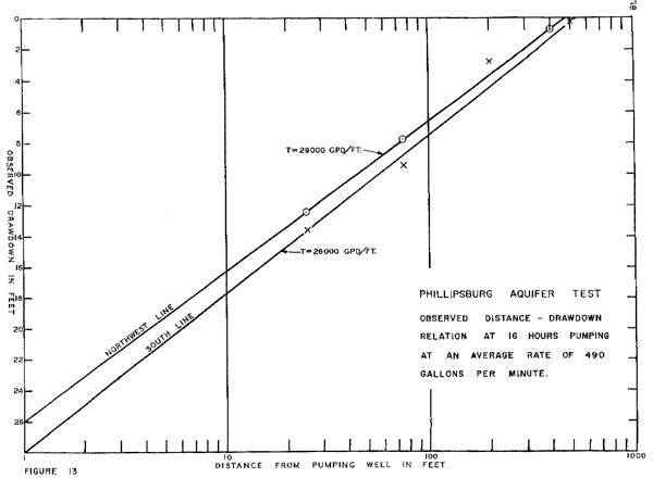
Figure D3 is an example of an application of the C-J in distance approach to the pumping-test data. The C-J in distance formula used in the Nuzman (1969) report was
T = 2.3Q/(2πΔsd)
where Δsd is drawdown over a log cycle in distance. The critical point is that this formula assumes that drawdown is small relative to the saturated thickness of the aquifer. However, that assumption is not valid here. For example, the drawdown at OW-25 Northwest is around 12.3 ft out of a total aquifer thickness of 28 ft. The validity of the C-J in distance formula is primarily a function of conditions between the two observation wells - in this case, the assumption of a small drawdown relative to the saturated thickness is not valid between those wells and the method cannot be used. Instead, the appropriate analysis method is the unconfined variant of the Thiem method:
T = [2.3Q log(75/25)]/(2π[(s1 - ((s1)2/2D)) - (s2 - ((s2)2/2D))]) where si is the drawdown at well i with 1 being OW-25 and 2 being OW-75, and D is the initial saturated thickness. This formula considers changes in saturated thickness and should be valid between OW-1 and OW-2 for both the south and northwest lines of wells at late times (i.e., after steady-shape conditions have been achieved [drawdown data are linear in the log of time]). When I applied this formula to the final drawdown points for OW-25 NW and OW-75 NW on Figure D2, I get a T of 87,500 gpd/ft, which is essentially the same as that obtained using the C-J in time formula.
The average of the two T estimates is approximately 86,000 gpd/ft. This converts to a T of 11,570 ft2/d and a K of 410 ft/d (28 ft saturated thickness). In terms of the units used in the Nuzman (1969) report, the K would be 3,090 gpd/ft2.
Additional reference:
Butler, J.J., Jr., 1998, Pumping tests in nonuniform aquifers--the radially symmetric case: Journal. of Hydrology, v. 101, no. 1/4, pp. 15-30.
Figure D1. Time-drawdown plot for the south observation wells in the 1968 pumping test of the alluvial aquifer of the North Fork of the Solomon River in Phillips County (from Nuzman, 1969).
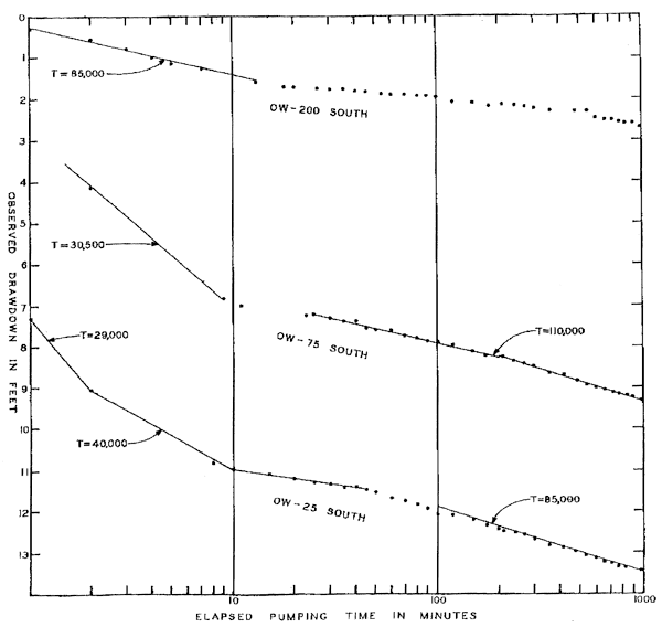
Figure D2. Time-drawdown plot for the northwest observation wells in the 1968 pumping test of the alluvial aquifer of the North Fork of the Solomon River in Phillips County (from Nuzman, 1969).
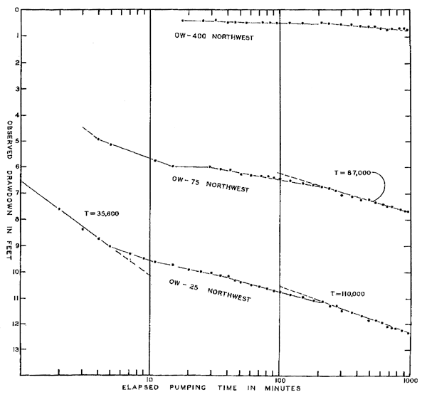
Figure D3. Distance-drawdown plot for the observation wells in the 1968 pumping test of the alluvial aquifer of the North Fork of the Solomon River in Phillips County (from Nuzman, 1969).
Kansas Geological Survey, Geohydrology
Placed online March 2, 2007
Comments to webadmin@kgs.ku.edu
The URL for this page is http://www.kgs.ku.edu/Hydro/Publications/2007/OFR07_4/index.html