Kansas Geological Survey, Open-file Report 2000-26
by
C. D. McElwee
Prepared for Presentation at
Spring AGU Meeting, Washington, DC
May 31, 2000
KGS Open-file Report 2000-26
Knowledge of the hydraulic conductivity distribution is of utmost importance in understanding the workings of an aquifer and in planning the consequences of any action taken upon that aquifer. For example, the effects of resource development or of contaminant remediation depend critically upon the in-situ hydraulic conductivity. Slug tests have been used extensively to measure hydraulic conductivity in the last fifty years since Hvorslev's work. Slug test responses can run the gamut from overdamped to underdamped. Until recently models were readily available for only the two extremes.
A general nonlinear model based on the Navier-Stokes equation, nonlinear frictional loss, non-Darcian flow, acceleration effects, radius changes in the wellbore, and a Hvorslev model for the aquifer has been developed (McElwee and Zenner, 1998). The nonlinear model has three parameters: beta which is related to radius changes in the water column, A which is related to the nonlinear head losses, and K the hydraulic conductivity. An additional parameter has been added representing the initial velocity of the water column at slug initiation, VEL0. We find that the model is quite robust in its estimates of K over varying conditions and allows a wide range of slug test data to be analyzed with a greater accuracy than traditional linear methods. The model covers the entire range of responses from overdamped to underdamped.
To obtain maximum accuracy in analyzing slug test data one should use a model that will seamlessly simulate responses for the overdamped region through the critically damped region and on into the underdamped region. This is particularly important when taking multilevel data sets at a site where the hydraulic conductivity changes dramatically from location to location. Multiple slug tests should be taken at a given location to test for nonlinear effects and to determine repeatability. This will allow some statistical measure of the experimental accuracy. As the hydraulic conductivity and the velocities in the wellbore increase, the nonlinear effects represented by the parameter A also increase. At some point the slug test response will become oscillatory as the hydraulic conductivity increases. The parameter beta represents a correction to the water column length caused by radius variations in the wellbore and is most useful in matching the oscillation frequency. Sensitivity analysis shows that in general beta and VEL0 have the lowest sensitivity and hydraulic conductivity usually has the highest, however, for very high K's the sensitivity to A may surpass that due to K. The sensitivities vary with hydraulic conductivity but we find the model to be robust with regard to estimates of hydraulic conductivity. Since oscillatory slug tests involve accelerations of the water column, we find that the pressure transducer responses are affected by these accelerations. For maximum accuracy of analysis, the model response must be corrected for acceleration before comparison to the transducer response.
Knowledge of the hydraulic conductivity distribution is of utmost importance in understanding the workings of an aquifer and in planning the consequences of any action taken upon that aquifer. For example, the effects of resource development or of contaminant remediation depend critically upon the in-situ hydraulic conductivity. Slug tests have been used extensively to measure hydraulic conductivity in the last fifty years since Hvorslev's work. Slug test responses can run the gamut from overdamped to underdamped. Until recently models were readily available for only the two extremes.
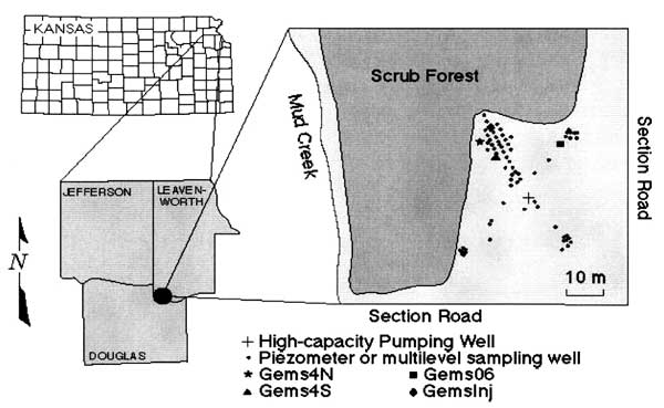
A field site, GEMS, in the Kansas River alluvium (coarse sand and gravel overlain by silt and clay) exhibits very high conductivities and nonlinear behavior for slug tests in the sand and gravel region. It is known from extensive drilling, sampling, and a tracer test that the hydraulic conductivity varies a great deal spatially. Over 70 wells have been completed at various depths. Slug tests have been performed in wells that are completed in the sand and gravel interval using a packer system with a piston for slug test initiation, allowing accurate determination of the initial head and starting time for the slug test.
Location map for the Geohydrologic Experimental and Monitoring Site (GEMS).
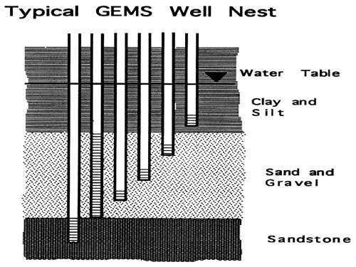
A typical well nest is shown in the next figure. Typically there is a fully screened well and several wells with short screens completed at various depths. In some nests we may have a well completed into the bedrock.
A general nonlinear model based on the Navier-Stokes equation, nonlinear frictional loss, non-Darcian flow, acceleration effects, radius changes in the wellbore, and a Hvorslev model for the aquifer has been developed.
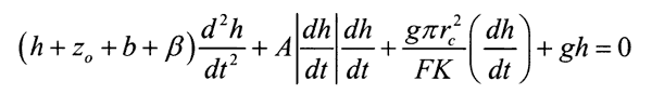
The nonlinear model has three parameters: β which is related to radius changes in the water column, A which is related to the nonlinear head losses, and K the hydraulic conductivity. An additional parameter has been added representing the initial velocity of the water column at slug initiation, VEL0. Normally VEL0 would be zero, but it appears that sometimes at initiation the water column obtains an initial velocity. Since in this work a piston was used for initiation, it is understandable how that might happen. We find that the model is quite robust in its estimates of K over varying conditions and allows a wide range of slug test data to be analyzed with a greater accuracy than traditional linear methods. The model covers the entire range of responses from overdamped to underdamped.
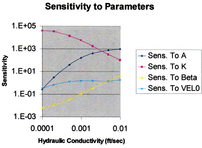
Sensitivity analysis is a formalism that allows the estimation of the effect on model response due to changing one parameter (McElwee, 1987). This can be combined with a model fitting routine to iteratively determine the set of parameters that give the best fit to experimental data. The sensitivity coefficient is defined as
![]()
which is a measure of how much the head (model output) changes when the parameter p is changed by a small amount. A sensitivity coefficient can be defined for each parameter, so if there are N parameters an NxN sensitivity matrix can be defined and used in the usual least squares fitting procedure to produce the following equation for parameter increments Δp
where Δh is the difference between experimental and model head and WU is the sensitivity matrix. The diagonal elements of the sensitivity matrix are a measure of the model sensitivity to a given parameter. The current model has four parameters (beta, A, K, and VEL0). The diagonal elements of the sensitivity matrix for these four parameters are plotted below. Sensitivity analysis shows that in general beta and VEL0 have the lowest sensitivity and hydraulic conductivity usually has the highest, however, for very high K's the sensitivity to A may surpass that due to K. The sensitivities vary with hydraulic conductivity but we find the model to be robust with regard to estimates of hydraulic conductivity.
Multiple slug tests should be performed at a given location to test for nonlinear effects and to determine if the tests are repeatable (Butler et al., 1996). As the hydraulic conductivity and the velocities in the wellbore increase, nonlinear effects represented by the parameter A will also increase. At some point the slug test response will become oscillatory as the hydraulic conductivity increases. If multiple slug tests with the same initial head are not very repeatable that implies there is noise in the data or that the well is changing characteristics. Noise with a time trend will be particularly troublesome for longer duration slug tests produced by low values of K. Wells can change effective K from one slug test to another if the well has not been properly developed. Multiple tests will also allow some statistical measure of the experimental accuracy. One can analyze the slug tests individually and calculate the average and the standard deviation of K or any other fitted parameter.
The three following examples are from wells at the GEM site and span the range from overdamped to underdamped slug test responses. In each case some normalized slug test plots with differing initial heads are shown to investigate nonlinear effects. Examples of repeat slug tests for a given initial head are also shown to look for noise or changing well characteristics. In two of the examples the individual slug tests have been analyzed to allow calculation of the average and standard deviation in K.
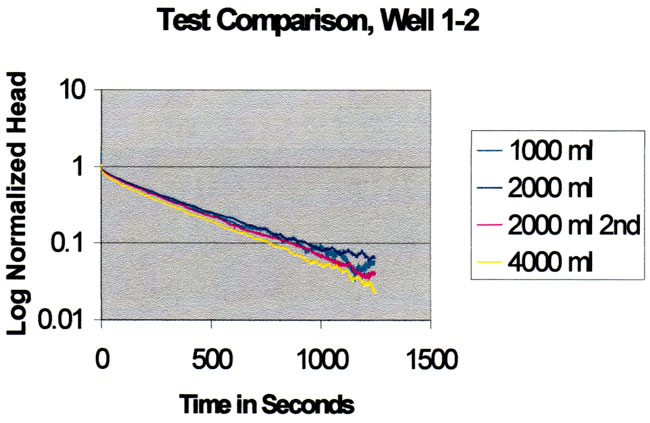
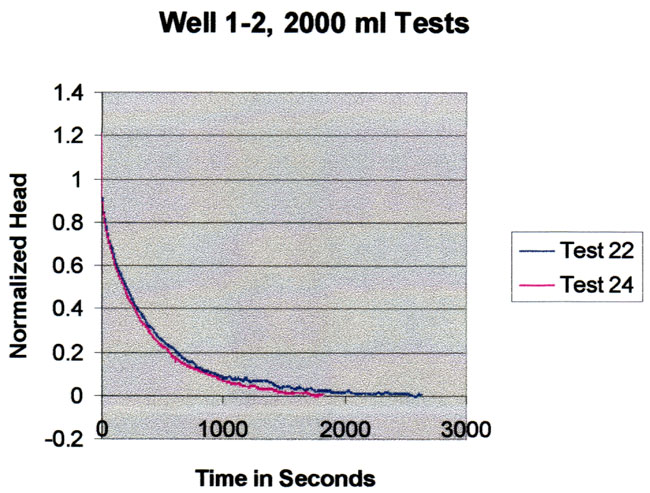
The figure below shows two repeat slug test responses for 2000 mi added to the well. The differences between the two curves represents the noise present during these tests. It appears that there was some varying time trends for the local water levels during these two tests. Since the tests were fairly lengthy, the effect is more pronounced than for shorter length tests.
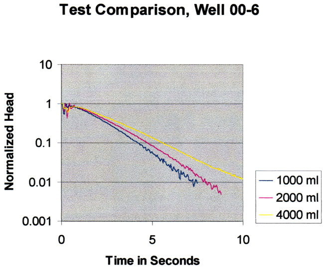
This well is completed at a depth of 42.4 feet with a screen length of 2.5 feet and in located in medium-grained material about 7.4 feet under the semiconfining layer at GEMS. This results in a moderate value for the hydraulic conductivity, however, the response is still an overdamped one. The plot here is also the usual Hvorslev form. There is a definite indication of nonlinear behavior here as the responses for differing initial heads are well separated. There is downward curvature in these responses in contrast to the previous well. The nonlinear model indicates that there is low sensitivity to beta and VEL0 but good sensitivity to K and A. The best fit for the suite of tests is K = 2.22x10⁻³ ft/sec and A = 14.19.
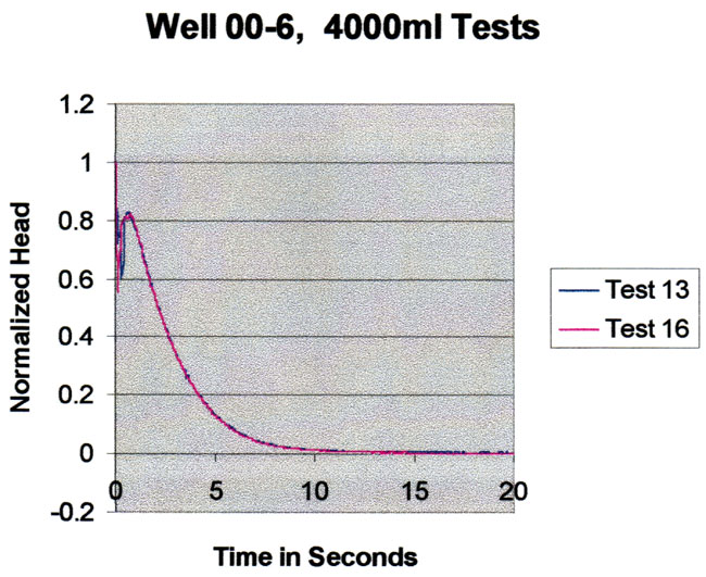
Repeat tests for 4000 ml added to the well are shown in the plot below. The tests basically fall on top of one another, indicating high reproducibility. These tests are over in about 10 seconds so they are not very susceptible to long term trends in local water levels.
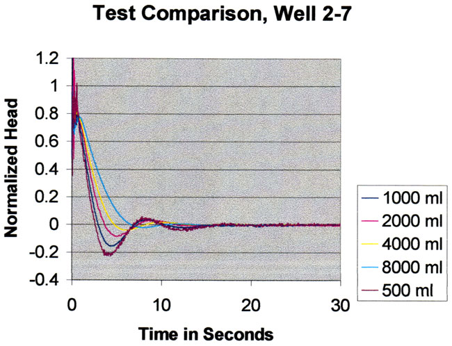
This well is completed at a depth of 56.4 feet with a screen length of 2.6 feet and is located in fairly coarse-grained material near the center of the alluvial aquifer at GEMS. In this environment there is a fairly high hydraulic conductivity and the response is definitely underdamped with significant oscillation. The plot is of normalized head versus time, which makes it appear that the oscillation is greater for smaller initial heads. However in fact, the negative oscillation is about the same magnitude for all responses. There is good separation of all responses indicating strong nonlinear effects. The nonlinear model indicates that there is moderate sensitivity to beta and VEL0 and strong sensitivity to A and K. The best fit for the suite of tests analyzed together is K = 4.8x10⁻³ ft/sec and A = 18.0. For 10 tests analyzed separately the average K is .00535 ft./sec with a standard deviation of .000743 ft/sec, which is a little less than 15% of the average value.
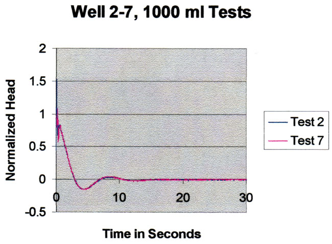
The figure below shows two repeat slug test responses for 1000 ml added to the well. The tests are nearly identical indicating high reproducibility and little evidence of local water level noise.
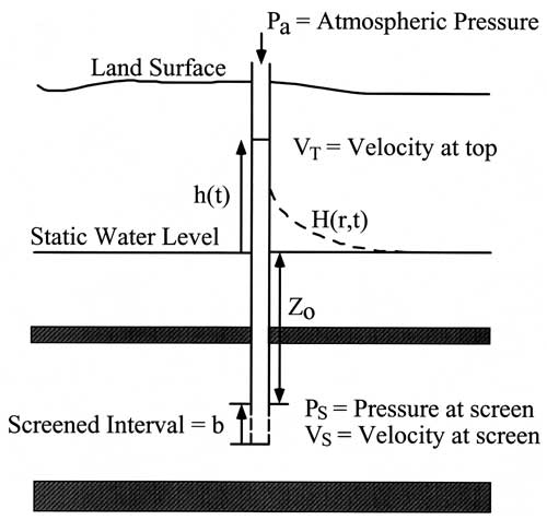
The parameter beta represents a correction to the water column length caused by radius variations in the wellbore and is most useful in matching the oscillation frequency and amplitude in wells with underdamped responses. For simple radius variations in the wellbore, the theoretical value for beta can be computed. Since oscillatory slug tests involve accelerations of the water column, we find that the pressure transducer responses are affected by these accelerations. Theoretically the correction for acceleration is given by
where he is the experimentally measured head, hm is the theoretical model head, Zs is the submergence of the pressure transducer, a is the acceleration of the water column, and g is the acceleration of gravity. For maximum accuracy of analysis, the model response must be corrected for acceleration before comparison to the transducer response. These two effects are illustrated in the following figures.
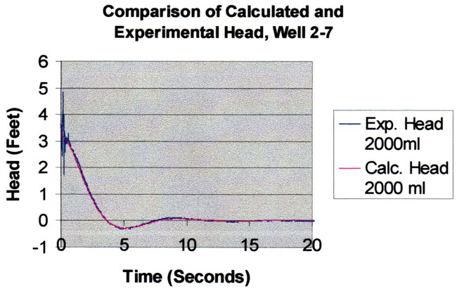
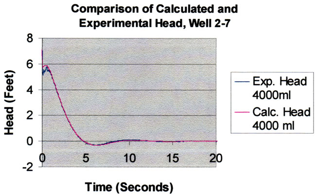
First of all, the results of fitting the nonlinear model to the 2000 ml and 4000 ml slug tests in well 2-7 are shown below. The response is underdamped and highly oscillatory and shows strong nonlinear effects. These two tests are matched well, indicating the model is describing the system well. The sum of squared errors for the fit is 6.87.
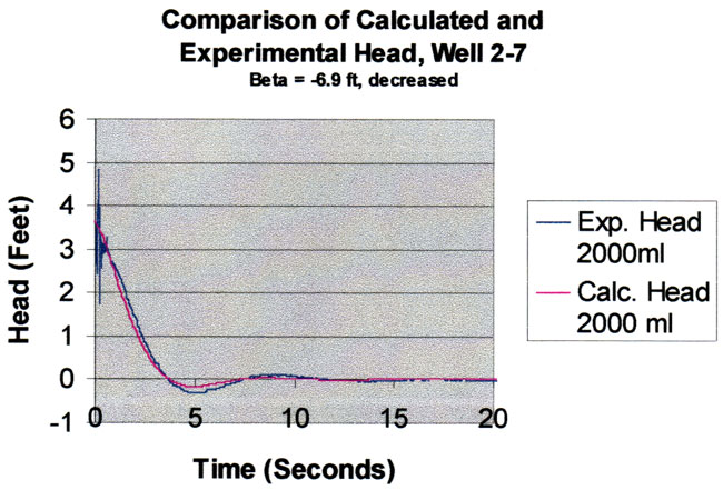
When the slug test responses are recalculated using a beta of -6.9 feet instead of the theoretical value of +6.9 feet (all other parameter values are held constant at their fitted values), the sum of squared errors increases to 30.78. The resulting response for the 2000 ml test is shown below. It is clear that the beta parameter is important in matching the amplitude and frequency of the oscillations.
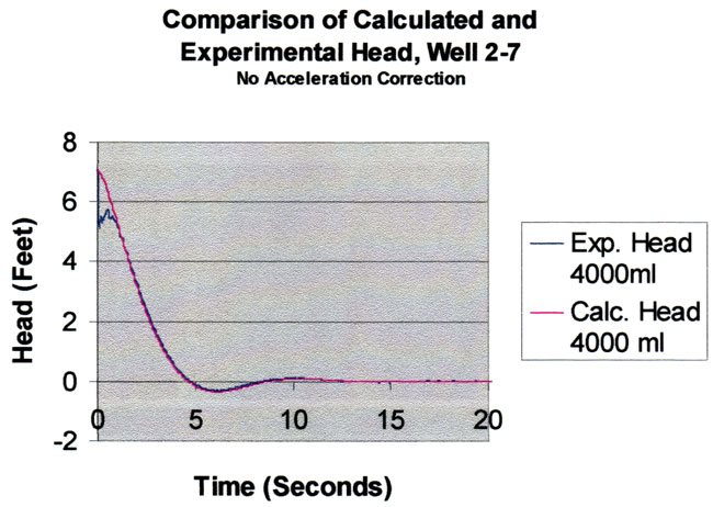
If the acceleration correction is turned off and the slug test responses are recalculated for the previously converged values of the parameters, the sum of squared errors increases to 13.18. A comparison of the model response without acceleration correction is compared to the 4000 ml slug test data in the figure below. It is clear that the early part of the experimental record is not as well produced as before. Although it is difficult to see, the fit with experimental data is not as good in those areas where the velocity is changing the most rapidly. Therefore, for maximum accuracy in fitting the data one should make the acceleration correction.
To obtain maximum accuracy in analyzing slug test data one should use a model that will seamlessly simulate responses for the overdamped region through the critically damped region and on into the underdamped region. This is particularly important when taking multilevel data sets at a site where the hydraulic conductivity changes dramatically from location to location. Multiple slug tests should be taken at a given location to test for nonlinear effects and to determine repeatability. This will allow some statistical measure of the experimental accuracy. As the hydraulic conductivity and the velocities in the wellbore increase, the nonlinear effects represented by the parameter A also increase. At some point the slug test response will become oscillatory as the hydraulic conductivity increases. The parameter beta represents a correction to the water column length caused by radius variations in the wellbore and is most useful in matching the oscillation frequency. Sensitivity analysis shows that in general beta and VEL0 have the lowest sensitivity and hydraulic conductivity usually has the highest, however, for very high K's the sensitivity to A may surpass that due to K. The sensitivities vary with hydraulic conductivity but we find the model to be robust with regard to estimates of hydraulic conductivity. Since oscillatory slug tests involve accelerations of the water column, we find that the pressure transducer responses are affected by these accelerations. For maximum accuracy of analysis, the model response must be corrected for acceleration before comparison to the transducer response.
Butler, J.J., Jr., McElwee, C.D., and Liu, W., 1996, Improving the quality of parameter estimates from slug tests: Ground Water, v. 34, no. 3, pp. 480-490.
Chirlin, G.R., 1989, A critique of the Hvorslev method for slug test analysis: The fully penetrating well: Ground Water Monitoring Review, v. 9, no. 2, pp. 130-138.
McElwee, C.D., 1987, Sensitivity analysis of ground-water models; in, Proceedings of the 1985 NATO Advanced Study Institute on Fundamentals of Transport Phenomena in Porous Media, edited by J. Bear and M.Y. Corapcioglu: Martinus Nijhoff, Dordrecht, Netherlands. pp. 751-817.
McElwee, C.D., and Zenner, M., 1998, A nonlinear model for analysis of slug-test data: Water Resources Research., v. 34, no. 1, pp. 55-66.
Kansas Geological Survey, Geohydrology
Placed online Nov. 20, 2007, original report dated May 2000
Comments to webadmin@kgs.ku.edu
The URL for this page is http://www.kgs.ku.edu/Hydro/Publications/2001/OFR00_26/index.html