Kansas Geological Survey, Open-file Report 1999-8
Prev page--Start, Deerfield Site ||
Next page--Dodge City Site, Conclusions
The Garden City site is located in Finney County approximately one quarter of a mile south of the Arkansas River just east of Highway 83 (Figure 24). The site consists of five wells screened over different vertical intervals in the alluvial and underlying High Plains aquifers. Table 3 provides well construction information for the site, while Table 4 provides the schedule and details of the slug tests performed at the site.
Figure 24--Location map for Garden City monitoring site
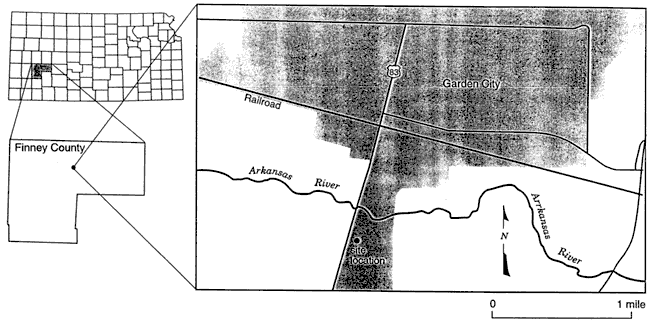
Table 3--Well construction information for wells at Garden City monitoring site.
| Well No. | Borehole Radius (ft) |
Casing Radius (ESR)1 (ft) |
Total Depth2 (ft) |
NSI3 (ft) |
Grout Interval4 (ft) |
|---|---|---|---|---|---|
| GCOW-1 | 0.250 | 0.103 (0.250) |
251 5 | 239-249 | 0-229 |
| GCOW-2 | 0.250 | 0.103 (0.250) |
209 5 | 197-207 | 0-188 |
| GCOW-3 | 0.312 6 | 0.103 (0.312) |
147 | 137-147 | 0-134 |
| GCOW-4 | 0.312 | 0.168 (0.312) |
88 | 78-88 | 0-74 |
| GCOW-5 | 0.458 | 0.168 (0.458) |
61 | 53-61 | 0-51 |
| 1--ESR or effective screen radius. In high-K formations, the effective screen radius may be closer to the nominal radius of the well screen (Butler, 1996). 2--depths are from top of casing in this and remaining columns 3--NSI = nominal screened interval 4--neat cement grout 5--depth includes a sump at bottom of screen 7--WWC-5 form has incorrect value of 0.250 ft. |
|||||
Table 4--Schedule and details of slug tests performed at the Garden City monitoring site
| Date | Test Well 1 |
Test No. |
H0* (ft) 2 |
%Rec 3 | H0/H0* 4 |
|---|---|---|---|---|---|
| 6/18/98 | GCOW-1 | 1 | 4.50 | 99.9 | 1.00 |
| 2 | 9.36 | 99.8 | 1.03 | ||
| 3 | 9.35 | 99.7 | 1.06 | ||
| 4 | 4.54 | 99.7 | 1.08 | ||
| 6/18/98 | GCOW-2 | 1 | 4.56 | 99.4 | 1.00 |
| 2 | 9.22 | 99.7 | 1.03 | ||
| 3 | 9.22 | 99.8 | 1.03 | ||
| 4 | 4.50 | 99.6 | 1.01 | ||
| 6/18/98 | GCOW-3 | 1 | 4.40 | 98.4 | 1.07 |
| 2 | 9.03 | ??5 | 1.04 | ||
| 3 | 9.26 | ??5 | 1.02 | ||
| 4 | 4.26 | 99.5 | 1.05 | ||
| 6/18/98 | GCOW-4 6 | 1 | 0.84 | 97.8 | 0.39 |
| 2 | 0.84 | 100.0 | 0.95 | ||
| 3 | 1.84 | 99.4 | 0.47 | ||
| 4 | 1.84 | 99.8 | 0.94 | ||
| 5 | 0.84 | 98.7 | 0.56 | ||
| 6/18/98 | GCOW-5 6 | 1 | 0.84 | 99.8 | 0.93 |
| 2 | 0.84 | 97.3 | 1.00 | ||
| 3 | 1.84 | 100.0 | 0.89 | ||
| 4 | 1.84 | 99.6 | 1.00 | ||
| 5 | 0.84 | 98.2 | 0.94 | ||
|
1--wells listed in order in which tests were performed; tests at wells GCOW 1-3 were initiated with the pneumatic method, while tests at wells GCOW 4-5 were initiated with solid slugs 2--expected H0 measured by air-pressure transducer or calculated from water displaced by solid slug in blank casing 3--percent recovery--relative measure of how close well had returned to static conditions prior to test initiation--one minus ratio of distance from static at time of test initiation over H0 (both based on water-pressure transducer readings) times 100 4--H0 measured at time of test initiation with water-pressure transducer over H0*--values greater than approximately 1.05 are a product of sensor noise and the methodology used to estimate H0 from the water-pressure transducer readings, while values less than about 0.95 may be an indication of a test initiation that was non-instantaneous relative to the formation response or water-pressure transducer readings that need to be adjusted for dynamic pressure effects 5--pump apparently turned on and off during this period making it difficult to estimate static conditions 6--noise associated with solid-slug initiation method made it difficult to obtain reliable estimates of H0/H0* |
|||||
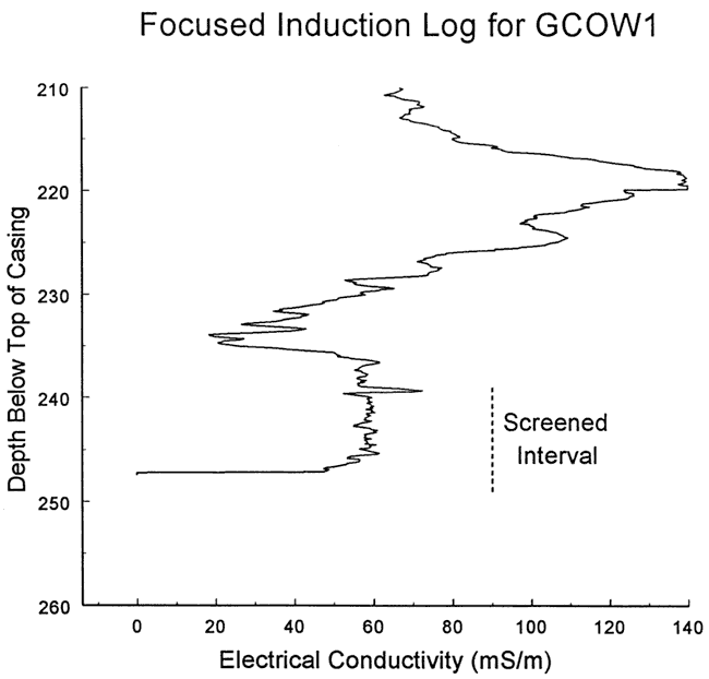
Four slug tests were performed at well GCOW-1 on June 18, 1998. Figure 25 is a plot of normalized head versus logarithm of time for this series of tests. As shown in the figure, response data from all four tests are oscillatory in nature. The plots for tests initiated with a large H0 are damped with respect to those for the other tests, indicating the presence of a head dependence. The near-coincidence of the response plots from tests initiated with similar H0 indicates that dynamic skin effects are quite small at this well. Test four was selected for analysis because of a slightly lower noise level than test one. Figure 26 displays the focused induction log in the vicinity of the test interval (no logging data available below screened interval).
Figure 25--Normalized head (H(t)/H0) versus the logarithm of time since test initiation for series of slug tests performed at well GCOW-1.
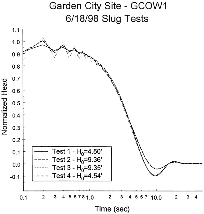
Figure 26--Focused induction log at well GCOW-1 for portions of the formation in the vicinity of the screened interval (spike at top of screened interval produced by casing centralizer).
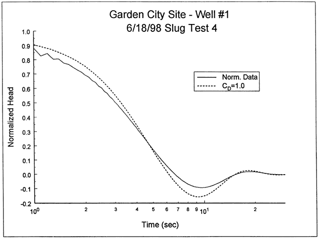
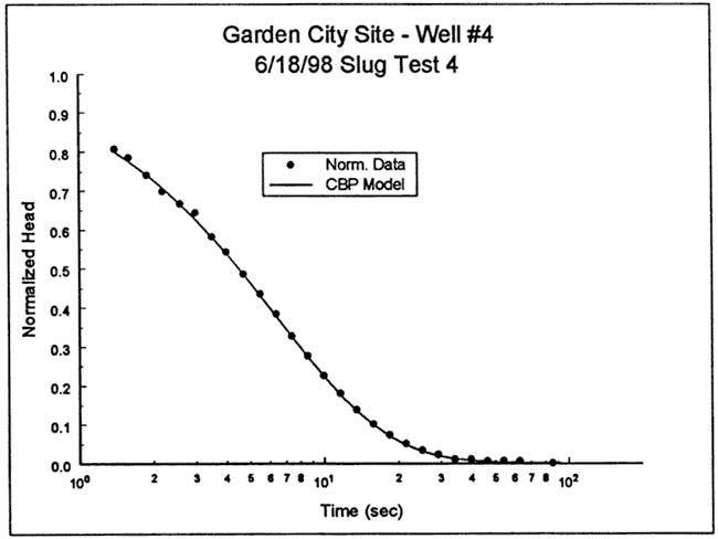
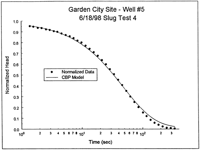
The response data from test four were analyzed with the high-K Hvorslev model, assuming that the head dependence was of little significance. Figure 27 is a plot of the normalized data from test four and a theoretical type curve (CD = 1.0, Le = 203.8 ft) from the high-K Hvorslev model. Because of the head dependence and additional nonidealities, the analysis was directed towards determining the type curve that bounds the test data. The CD = 1.0 type curve is considered a reasonable bound on the test data. The differences between the type curve and the response data at early times are most probably a function of dynamic pressure effects and the head dependence. The high-K Hvorslev model has two variants: 1) top and bottom impermeable boundaries do not influence test responses (equation (8.9c) of Butler (1997), usual situation assumed in practice); and 2) well screened up against an impermeable boundary (equation (8.9c) of Butler (1997) with (1/ψ) replacing (1/(2ψ)) . Although not shown in the log of Figure 26, GCOW-1 is screened up against a sandstone bedrock. Thus, the second variant of the high-K Hvorslev model was used here. Substituting a CD value of 1.0, an effective column length (Le) of 203.8 ft, and the well construction parameters of Table 3 into the modified form of equation (8.9c) of Butler (1997) produces a K estimate of 127 ft/day, a value that is quite reasonable for a test interval consisting of sand and gravel. Note that the effective column length of 203.8 ft is within 12.1 ft (6.3%) of what would be expected from the depth to water measurement and well construction information, lending further credence to the analysis results. Analyses using other methods described in Butler (1997) produced similar results.
Figure 27--Normalized head (H(t)/H0) versus log time plot for test 4 at GCOW-5 and a bounding theoretical type curve from the high-K Hvorslev model.
As noted in Table 3, there is some question about the effective screen radius in high-K intervals, which translates into uncertainty in the K estimate. The K estimate of 127 ft/day was obtained assuming that the effective screen radius was equal to the borehole radius. Since the hydraulic conductivity of the filter pack is probably not much greater than that of the formation, the nominal outer radius of the well screen might be a more appropriate quantity for the effective screen radius. In that case, a K estimate of 153 ft/day is obtained. Thus, the K estimate is between 127 and 153 ft/day, and most likely lies towards the upper end of that range.
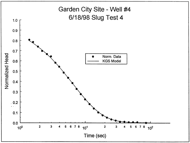
Four slug tests were performed at well GCOW-2 on June 18, 1998. Figure 28 is a plot of normalized head versus logarithm of time for this series of tests. As shown in the figure, a small amount of head dependence was observed, which was assumed negligible for analysis purposes. There was no evidence of dynamic skin effects at this well. Test one was selected for analysis but test four would have been an equally viable alternative. Figure 29 displays the focused induction log in the vicinity of the test interval.
Figure 28--Normalized head (H(t)/H0) versus the logarithm of time since test initiation for series of slug tests performed at well GCOW-2.
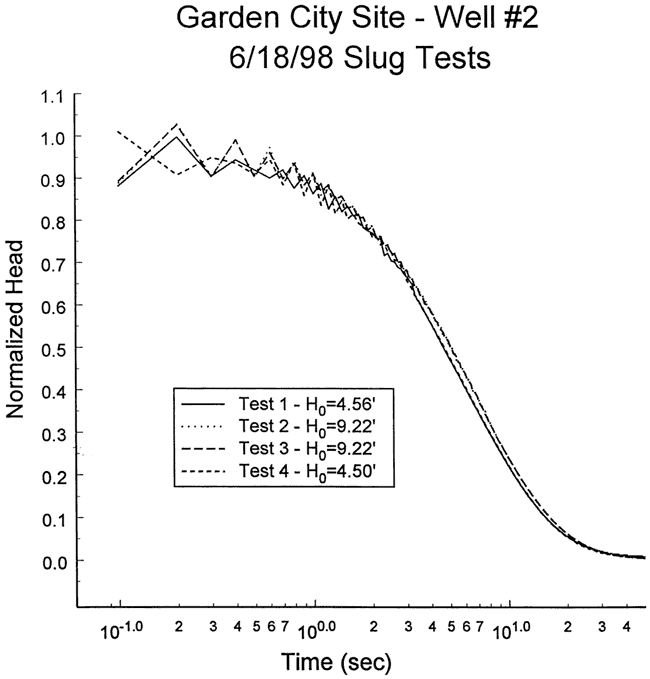
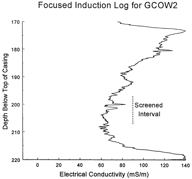
Figure 29--Focused induction log at well GCOW-1 for portions of the formation in the vicinity of the screened interval at GCOW-2.
The response data were first analyzed with the fully penetrating well model of Cooper et al. Figure 30 is a plot of the normalized data and the best-fit Cooper et al. type curve for a specific storage value at the lower end of the range of physical plausibility (Ss equals 1.7x10⁻⁶ ft-1). In this case, a reasonable match could not be obtained with the Cooper et al. model. A significant component of vertical flow or a low-conductivity well skin were considered the most likely explanations for the deviation observed in Figure 30.
Figure 30--Normalized head (H(t)/H0) versus log time plot for test 1 at GCOW-2 and the best-fit Cooper et al. type curve (Ss equals 1.7x10⁻⁶ ft-1).
The response data Vere next analyzed with the KGS model for partially penetrating wells (layer thickness = 34 ft, impermeable unit 13 ft above top of screen). Because of the small degree of head dependence observed in the test data, specific storage was assumed fixed for the analysis (Ss equals 1.7x10⁻⁶ ft-1). Figure 31 is a plot of the normalized data and the KGS model type curve (K = 23 ft/day). Although the fit is noticeably better than that obtained with the Cooper et al. model, there is still a systematic deviation between the test data and the type curve. This deviation could not be removed by repeating the analysis with physically implausible values of specific storage.
Figure 31--Normalized head (H(t)/H0) versus log time plot for test 1 at GCOW-2 and the best-fit KGS model type curve (Ss equals 1.7x10⁻⁶ ft-1).
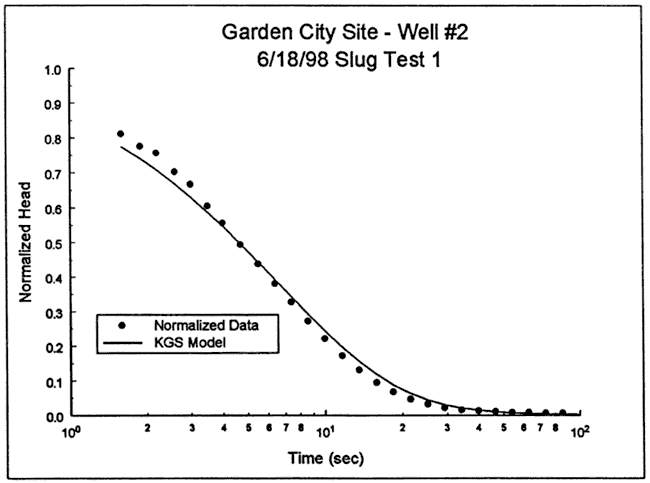
Despite analyses using more sophisticated models, a satisfactory explanation for the deviation shown in Figure 30 could not be found. Most likely, this deviation is a product of a number of factors including a small degree of head dependence, formation heterogeneities, and, possibly, a low-conductivity well skin. Thus, the K estimate of 23 ft/day should be considered as a conservative lower bound on the hydraulic conductivity of the formation in the vicinity of the screened interval at well GCOW-2.
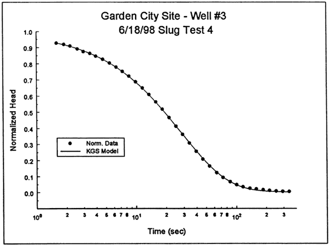
Four slug tests were performed at well GCOW-3 on June 18, 1998. Figure 32 is a plot of normalized head versus logarithm of time for this series of tests. Note that tests two and three did not return to static conditions defined on the basis of pre-test heads. Apparently, nearby pumping activity changed the static heads for these tests. When static conditions and H0 are defined on the basis of post-test heads, Figure 33 shows that the normalized plots for the four tests are in much better agreement. The similarity between the four tests shown on Figure 33 indicates that nonlinear mechanisms and dynamic skin effects can be ignored at this well. Test four was selected for analysis but test one was an equally viable alternative. Figure 34 displays the focused induction log in the vicinity of the test interval.
Figure 32--Normalized head (H(t)/H0) versus the logarithm of time since test initiation for series of slug tests performed at well GCOW-3.
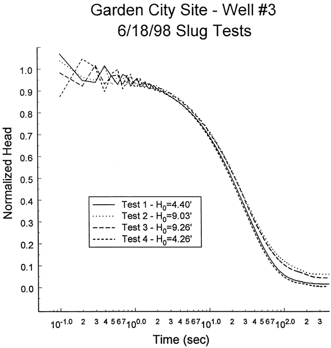
Figure 33--Normalized head (H(t)/H0) versus the logarithm of time since test initiation for series of slug tests performed at well GCOW-3, tests two and three adjusted as described in text.
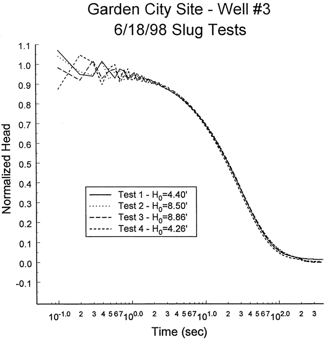
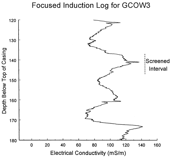
Figure 34--Focused induction log at well GCOW-1 for portions of the formation in the vicinity of the screened interval at GCOW-3.
The response data were first analyzed with the fully penetrating well model of Cooper et al. Figure 35 is a plot of the normalized data and the best-fit Cooper et al. type curve for a specific storage value at the lower end of the range of physical plausibility (Ss = 1.1x10⁻⁶ ft-1) . As shown in the figure, a reasonable match could not be obtained using a physically plausible value of specific storage. The failure to obtain an acceptable match within the range of physically plausible parameter values is most probably a product of a significant component of vertical flow.
Figure 35--Normalized head (H(t)/H0) versus log time plot for test 1 at GCOW-3 and the best-fit Cooper et al. type curve (Ss equals 1.1x10⁻⁶ ft-1).
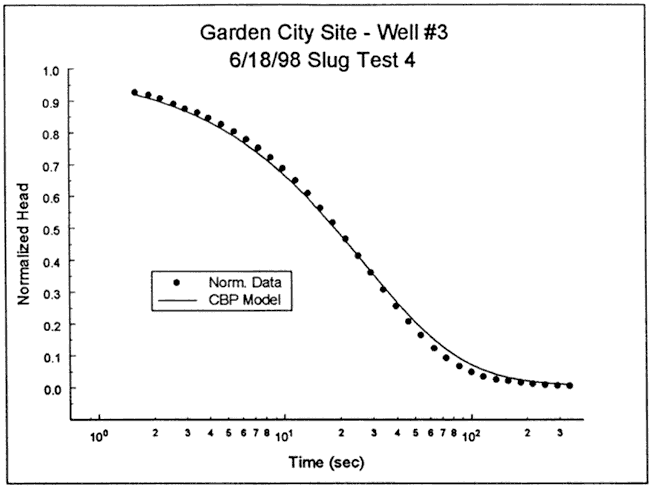
The response data were next analyzed with the KGS model for partially penetrating wells (layer thickness ≥ 52 ft, impermeable unit 26 ft below bottom of screen). Figure 36 is a plot of the normalized data and the best-fit KGS model type curve (K = 4.8 ft/day, Ss = 5.8x10⁻⁶ ft-1). The excellent fit obtained with a physically plausible value of specific storage provides further support for the assumption that the deviation seen on Figure 35 is a product of a significant component of vertical flow. Note that these data were also analyzed with the Hvorslev model, resulting in a K estimate within 2% of that found using the KGS model.
Figure 36--Normalized head (H(t)/H0) versus log time plot for test 1 at GCOW-3 and the best-fit KGS model type curve (Ss equals 5.8x10⁻⁶ ft-1).
Five slug tests were performed at well GCOW-4 on June 18, 1998. Figure 37 is a plot of normalized head versus logarithm of time for this series of tests. The solid slug initiation method introduced considerable noise into the test data. This noise, coupled with uncertainty about start times and static levels, was assumed to be responsible for the differences between the tests shown on Figure 37. The impact of nonlinear mechanisms and dynamic skin effects was assumed negligible. The solid slug was removed from the well in tests two and four, producing H0/H0* ratios close to one, so these tests were considered the best for analysis. Test four was selected because the larger H0 produced a lower degree of noise in the normalized data. Figure 38 displays the focused induction log in the vicinity of the test interval.
Figure 37--Normalized head (H(t)/H0) versus the logarithm of time since test initiation for series of slug tests performed at well GCOW-4.
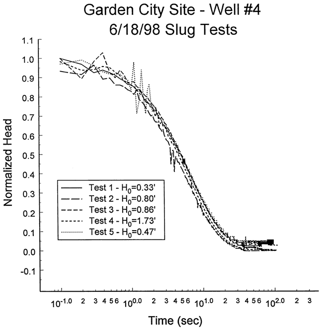
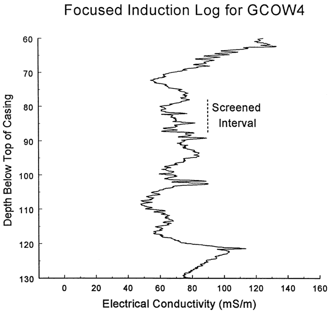
Figure 38--Focused induction log at well GCOW-1 for portions of the formation in the vicinity of the screened interval at GCOW-4.
The response data were first analyzed with the fully penetrating well model of Cooper et al. Figures 39 and 40 are plots of the normalized data and the best-fit Cooper et al. type curve for two specific storage values (Ss = 2.9x10⁻⁶ ft-1 and 2.9x10⁻²⁰ ft-1 , respectively). As shown in the figures, a reasonable match could only be obtained using a physically implausible value of specific storage. The failure to obtain an acceptable match within the range of physically plausibility is most probably a product of a significant component of vertical flow.
Figure 39--Normalized head (H(t)/H0) versus log time plot for test 1 at GCOW-4 and the best-fit Cooper et al. type curve (Ss equals 2.9x10⁻⁶ ft-1).
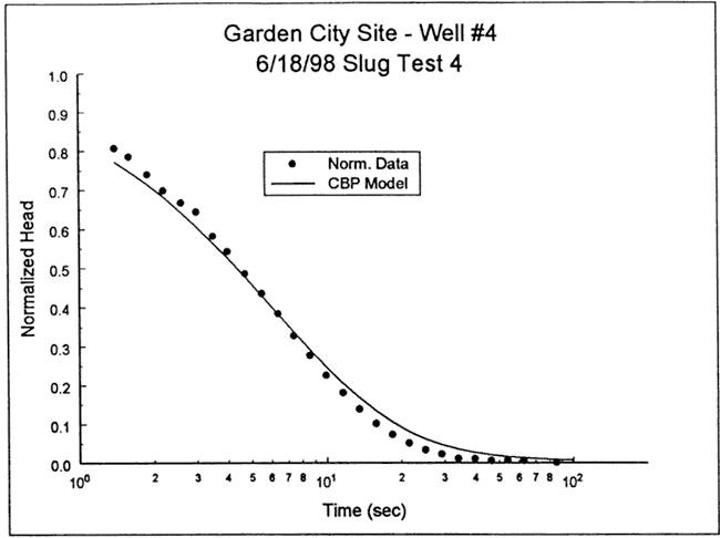
Figure 40--Normalized head (H(t)/H0) versus log time plot for test 1 at GCOW-4 and the best-fit Cooper et al. type curve (Ss equals 2.9x10⁻²⁰ ft-1).
The response data were next analyzed with the KGS model for partially penetrating wells (layer thickness of 58 ft, impermeable unit 15 ft above top of screen). Figure 41 is a plot of the normalized data and the best-fit KGS model type curve (K = 58 ft/day) for a specific storage value fixed at 2.9x10⁻⁶ ft-1. The fit could be improved a small amount by decreasing the specific storage, but the K value changed by less than 10%. In this case, the improved fit produced by decreasing the specific storage was attributed to the possible presence of a layer of higher hydraulic conductivity a short distance below the screened interval. This layer, which is not apparent from the focused induction log, is quite pronounced on the natural gamma log. Note that these data were also analyzed with the Hvorslev model, resulting in a K estimate within 7% of that obtained using the KGS model.
Figure 41--Normalized head (H(t)/H0) versus log time plot for test 1 at GCOW-4 and the best-fit KGS model type curve (Ss equals 2.9x10⁻⁶ ft-1).
Five slug tests were performed at well GCOW-5 on June 18, 1998. Figure 42 is a plot of normalized head versus logarithm of time for this series of tests. The solid slug initiation method introduced considerable noise into the test data. This noise, coupled with uncertainty about start times and static levels, was assumed to be responsible for the differences between the tests shown on Figure 42. Since tests one, four and five essentially coincided, nonlinear mechanisms and dynamic skin effects were assumed negligible. Test four was selected for analysis because the larger H0 produced a lower degree of noise in the normalized data. Figure 43 displays the focused induction log in the vicinity of the test interval.
Figure 42--Normalized head (H(t)/H0) versus the logarithm of time since test initiation for series of slug tests performed at well GCOW-5.
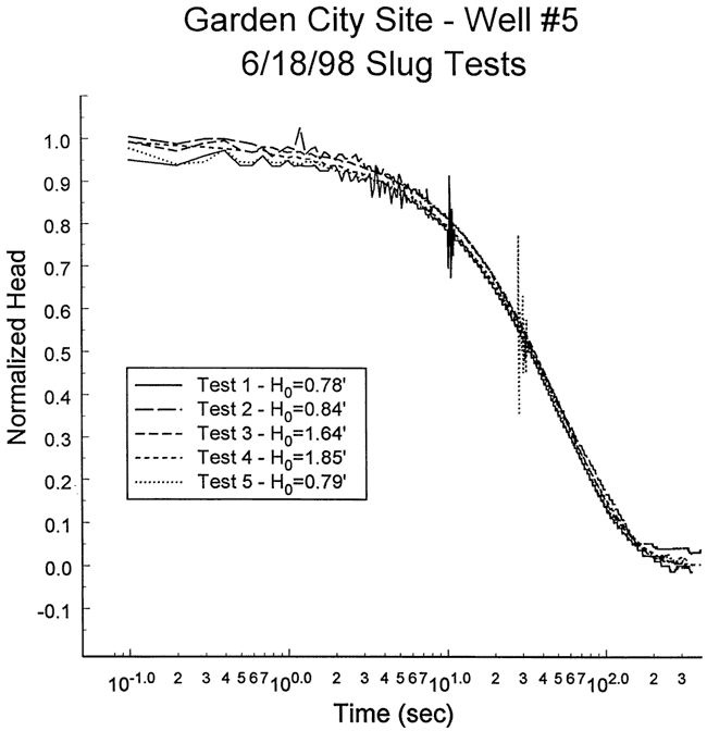
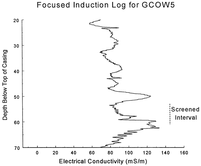
Figure 43--Focused induction log at well GCOW-1 for portions of the formation in the vicinity of the screened interval at GCOW-5.
The response data were first analyzed with the fully penetrating well model of Cooper et al. Figure 44 is a plot of the normalized data and the best-fit Cooper et al. type curve for a specific storage value at the lower bound of physical plausibility (Ss = 1.7x10⁻⁶ ft-1). There is a clear systematic deviation between the Cooper et al. model and the test data. In this case, a reasonable match could not be obtained with the Cooper et al. model using any specific storage value. The failure to obtain an acceptable match could be a product of a low-conductivity well skin or a significant component of vertical flow.
Figure 44--Normalized head (H(t)/H0) versus log time plot for test 1 at GCOW-5 and the best-fit Cooper et al. type curve (Ss equals 1.7x10⁻⁶ ft-1).
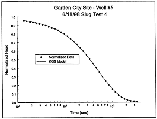
The focused induction log of Figure 43 shows a zone of higher electrical conductivity immediately above the screened interval. However, natural gamma logs of that zone at nearby wells indicate that it may not be a continuous clay unit. Thus, there may be no barriers to vertical flow between the top of the screened interval and the water table (30.5 ft below the top of the casing). The response data were therefore analyzed with the unconfined form of the KGS model for partially penetrating wells (layer thickness of 32.5 ft, top of screen 22.5 ft below water table). Figure 45 is a plot of the normalized data and the best-fit KGS model type curve (K=8.1 ft/day, Ss = 1.4x10⁻⁵ ft-1), illustrating the excellent match that was obtained. The hydraulic conductivity estimate from the KGS model was supported by an analysis with the Bouwer and Rice model, which produced a K estimate within 7% of that obtained using the KGS model. Since there is some question about the continuity of the layer of higher electrical conductivity above the top of the screen, the K estimate should be considered a conservative lower bound on the hydraulic conductivity of the formation in the vicinity of the test interval at GCOW-5.
Figure 45--Normalized head (H(t)/H0) versus log time plot for test 1 at GCOW-5 and the best-fit KGS model type curve (Ss equals 1.4x10⁻⁵ ft-1).
Prev page--Start, Deerfield Site || Next page--Dodge City Site, Conclusions
Kansas Geological Survey, Geohydrology
Placed online Dec. 6, 2007; original report dated Dec. 1999
Comments to webadmin@kgs.ku.edu
The URL for this page is http://www.kgs.ku.edu/Hydro/Publications/1999/OFR99_08/page2.html