Kansas Geological Survey, Open-file Report 98-15B
KGS Open File Report 98-15B
August 1998
The complete report is available as an Adobe Acrobat PDF file (388 kB).
A series of slug tests were performed by the Kansas Geological Survey in the monitoring wells in the Dakota well field of the city of Hays in Ellis County, Kansas in June of 1997. The major objective of this test program was to assess the suitability of the monitoring wells for use as observation wells in pumping tests. These slug tests demonstrated that the hydraulic connection with the Dakota sands was good enough for this purpose at all five wells. Although tests at one well (MD-1) indicated the presence of a low-permeability well skin, that well is relatively far from the nearest pumping well, so the skin should have little to no impact on drawdown during a pumping test. Tests at two wells (MD-5 and MD-6) indicated that the annular seals at those wells may be incomplete. This condition, however, should not affect the suitability of these wells for use as observation wells in pumping tests. Responses at four of the five wells were oscillatory in nature, a product of the long column of water above the screened interval, and required use of recently developed approaches for data analysis. The hydraulic conductivity estimates determined from this series of slug tests ranged from 4-13 ft/day. These values should be considered lower bounds on the hydraulic conductivity of the Dakota sands in the vicinity of the monitoring wells because of uncertainty about the effective screen length and the degree of anisotropy.
A series of slug tests were performed by the Kansas Geological Survey (KGS) in the monitoring wells in the Dakota well field of the city of Hays in Ellis County, Kansas in June of 1997. This work was done as part of an extension of the Dakota Aquifer Program, a multi-year research effort of the KGS directed at developing an understanding of the hydrologic, water-quality, and water-resources-management ramifications of increased utilization of the Dakota aquifer in central and western Kansas (Macfarlane et al., 1990). This extension of the Dakota Aquifer Program was funded by the city of Hays for the specific purpose of evaluating the long-term effect of water-resources development on the Dakota aquifer in the vicinity of the city's Dakota well field. P. Allen Macfarlane of the Geohydrology Section of the KGS served as the principal investigator for this project.
The slug tests that are the subj ect of this report were performed to assess the suitability of the monitoring wells for use as observation wells in pumping tests in the Dakota well field. The major focus of this assessment was on the degree of hydraulic connection between the monitoring wells and the Dakota sands. This report describes the procedures used for the performance and analysis of these slug tests. Approximately a month after the completion of the tests described in this report, two multi-day pumping tests were performed in the Dakota well field using the monitoring wells as observation wells. The performance and analysis of those pumping tests, along with details concerning the hydrogeology of the well field and its vicinity, are described in separate reports.
The location of the Dakota well field is in Ellis County, just south of the city of Hays, Kansas. Figure 1 shows the position of the well field relative to the city of Hays, and the distribution of pumping and monitoring wells within the well field. The slug tests that are the subject of this report were performed at the monitoring wells (wells with "MD" prefix on Figure 1). Table 1 provides well construction information for each of these wells.
Figure 1--Location map for the Dakota well field of the city of Hays (pumping wells labelled with prefix "D" and monitoring wells labelled with prefix "MD")
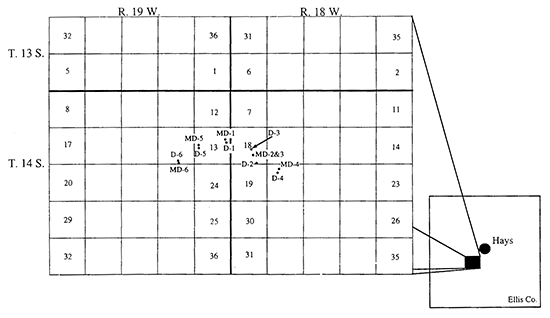
Table 1--Well construction information for monitoring wells in Dakota well field of the city of Hays.
| Well No. | Borehole Radius1 |
Casing Radius (ESR)2 |
Total Depth3 |
NSI4 | Sand Thickness5 |
Grout Interval |
|---|---|---|---|---|---|---|
| MD-1 | 0.333 | 0.081 (0.333) |
557 | 472-557 | 37 | 0-30 360-400 |
| MD-2&3 | 0.333 | 0.081 (0.333) |
496 | 425-435 455-495 |
46 | 0-30 260-280 360-380 |
| MD-4 | 0.333 | 0.081 (0.333) |
475 | 407-475 | 133 | 0-30 295-328 |
| MD-5 | 0.333 | 0.081 (0.333) |
no info.6 |
no info.6 |
88 | no info.6 |
| MD-6 | 0.333 | 0.081 (0.333) |
548 | 486-502 512-547 |
30 | 0-30 400-4307 |
| 1 - units for information in this and remaining columns are ft. 2 - ESR--effective screen radius 3 - depths are from land surface in this and remaining columns 4 - NSI--nominal screened interval 5 - estimates provided by P. Allen Macfarlane 6 - no WWC-5 form available for this well (P. Allen Macfarlane, personal communication) 7 - WWC-5 form states that grout extends to a depth of 530 ft. This is undoubtedly a typographical error, so 430 ft is assumed to be the correct figure. |
||||||
This program of slug tests was carried out following a recently defined set of guidelines for the design, performance and analysis of slug tests (Butler et al., 1996; Butler, 1997). These guidelines were the product of a multi-year KGS research effort directed at improving slug-test methodology. The pneumatic method (Butler, 1997) was used for test initiation at all five monitoring wells. This method involves placing an air-tight well-head apparatus (Figure 2) on top of the well and pressurizing the air column in the sealed well casing. This pressurization produces a depression of the water level in the well as water is driven out of the well and into the formation in response to the increased pressure in the overlying air column. The water level continues to drop until the magnitude of the total decrease in the pressure head of the water equals the magnitude of the total increase in the pressure head of the air column. At that point, the well has returned to static conditions (i.e. a pressure transducer in the water column has the same reading as prior to pressurization), and the test can be initiated by a very rapid depressurization of the air column using the release valve shown in Figure 2. A slug test initiated in this manner produces a flow of water into the well. Since the depth to water exceeded 200 ft at all five monitoring wells, complete depressurization of the air column took several seconds. Figure 3 presents normalized head (head relative to static normalized by the magnitude of the initial displacement (H0)) versus the logarithm of time since test initiation plots for slug tests performed at three of the monitoring wells. The oscillations in the first three to four seconds of the tests shown on Figure 3 are a product of pressure disturbances produced by the non-instantaneous depressurization of the air column. Similar early-time oscillations were seen in all of the tests described in this report. Since these oscillations were a product of the initiation method, and not of the properties of the formation, they were ignored during the analysis of the response data.
Figure 2--Hypothetical cross section depicting a well at which the pneumatic method is being used for test initiation (Butler, 1997).
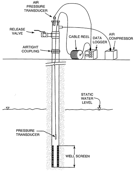
Figure 3--Normalized head (H(t)/H0, where H(t) is measured deviation from static and H0 is magnitude of the initial displacement) versus the logarithm of time since test initiation for slug tests at three monitoring wells in the Dakota well field.
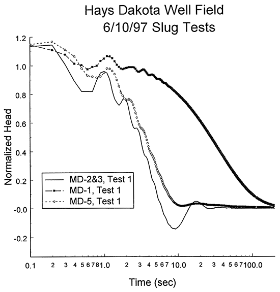
Table 2 shows the schedule and details of the slug tests performed in the Dakota well field. At least three tests were performed at each well following the guidelines of Butler et al. (1996) and Butler (1997). The initial displacement (H0) was varied by close to a factor of two during the series of tests at each well in order to assess the importance of nonlinear mechanisms. In addition, an attempt was made to perform at least two of the tests using approximately equal H0 to assess the significance of dynamic skin effects. The fifth column in Table 2 is a relative measure of how close the well had returned to static conditions prior to depressurization of the air column. As shown in the table, recovery exceeded 95% in most cases. Butler (1997) demonstrated that such a small degree of incomplete recovery (less than 5% in most cases) can be ignored for practical applications. The sixth column in Table 2 is the ratio recommended by Butler (1997) for assessing the relative speed of test initiation. Although Figure 3 indicates that the pneumatic method did not strictly satisfy the instantaneous-initiation assumption required for some theoretical slug-test models, the values given in column six of Table 2 indicate that test initiation can be considered instantaneous relative to the response of the Dakota sands in virtually all cases. Note that since Table 2 indicates that the ratio of H0 over H0* was close to one for all tests, no distinction is made between H0 and H0* for the remainder of this report.
Table 2--Schedule and details of slug tests performed in Dakota well field of the city of Hays.
| Date | Test Well1 |
Test No. |
H0* (ft)2 |
%Rec3 | H/H0* 4 |
|---|---|---|---|---|---|
| 6/10/1997 | MD-2&3 | 1 | 5.32 | 98.9 | 1.07 |
| 2 | 10.24 | 98.9 | 1.01 | ||
| 3 | 10.31 | 98.9 | 1.01 | ||
| 6/10/1997 | MD-1 | 1 | 8.91 | 95.55 | 1.03 |
| 2 | 4.81 | 92.86 | 1.06 | ||
| 3 | 8.79 | 91.96 | 1.03 | ||
| 6/10/1997 | MD-5 | 1 | 6.68 | 92.25 | 1.05 |
| 2 | 3.25 | 95.66 | 1.21 | ||
| 3 | 8.89 | 97.36 | 1.02 | ||
| 6/10/1997 | MD-6 | 1 | 12.74 | 95.25 | 0.91 |
| 2 | 11.60 | 99.2 | 0.95 | ||
| 3 | 11.77 | 99.6 | 0.96 | ||
| 4 | 7.43 | 99.4 | 0.99 | ||
| 6/11/1997 | MD-4 | 17 | 11.07 | 98.65 | 1.01 |
| 2 | 10.75 | 99.9 | 1.03 | ||
| 3 | 10.42 | 99.7 | 1.02 | ||
| 4 | 6.25 | 99.5 | 0.93 | ||
| 1 - wells listed in order in which tests were performed 2 - expected H0 measured by air-pressure transducer 3 - percent recovery - relative measure of how close well had returned to static conditions prior to test initiation - one minus ratio of distance from static at time of test initiation over H0 (both based on water-pressure transducer readings) times 100 4 - H0 measured at time of test initiation with water-pressure transducer over expected H, measured with air-pressure transducer--values greater than approximately 1.05 are a product of sensor noise and the methodology used to estimate H0 from the water-pressure transducer readings, while values less than about 0.95 may be an indication of a test initiation that was non-instantaneous relative to the formation response 5 - H0 value determined from water-pressure transducer may be in error due to thermal effects and well development accompanying test 6 - small air leak somewhere in well and well-head apparatus affected H0 reading 7 - significant portions of response data inadvertently deleted during transfer of data from datalogger to laptop computer |
|||||
For all the slug tests described in this report, changes in water level were measured using a pressure transducer (an In-Situ PXD-261 series 0-20 psig transducer) connected to a data logger (Campbell Scientific CR500 data logger). Air pressure within the sealed casing was monitored using a pressure transducer (an Instrumentation Northwest PS9000 series 0-30 psig transducer) and an analog pressure gauge (Davis Instruments Model 1082 series 0-30 psig gauge). casing pressurization was accomplished using a gasoline-powered air compressor.
The slug-test response data were analyzed by comparing the data to theoretical models that were thought to closely resemble the test configuration. In this work, two theoretical models of slug tests in confined aquifers were used: 1) the model of Cooper et al. (1967) for slug tests in fully penetrating wells in confined aquifers; and 2) the linearized variant of the model of McElwee et al. (Butler, 1997; McElwee and Zenner, 1998) for oscillatory slug tests in wells in confined aquifers. In addition to approaches based on theoretical slug-test models, the approximate deconvolution method of Peres et al. (1989) was also utilized. As explained by Butler (1997), this method involves transforming the slug test response data into the equivalent drawdown that would have been produced by a constant rate of pumping at the test well. The equivalent drawdown is then analyzed with the Cooper-Jacob semilog method for constant-rate pumping tests in confined aquifers (Kruseman and de Ridder, 1990). The approximate deconvolution method was used in this work because of its superiority in cases where low-permeability well skins are affecting the response data. In all cases, the general strategy for the analysis followed the guidelines presented in Chapter 13 of Butler (1997). Analyses using the Cooper et al. model were performed with SUPRPUMP, an automated well-test analysis package developed at the Kansas Geological Survey (Bohling et al., 1990; Bohling and McElwee, 1992), while analyses using the linearized variant of the McElwee et al. model involved graphical comparisons of data plots with type curves generated using the Mathcad software package (MathSoft, 1997). Analyses with the approximate deconvolution method of Peres et al. were performed using the DERIV program of Spane and Wurstner (1993) to compute the equivalent drawdown, and linear regression routines in the Axum software package (MathSoft, 1996) to compute the best-fit straight line for the Cooper-Jacob semilog method. Note that static water levels at all five monitoring wells were over 100 ft above the top of the Dakota sands, so only models for confined aquifers were considered here.
The primary parameter of interest for the test program described in this report was hydraulic conductivity. A considerable amount of research (e.g., Cooper et al., 1967; McElwee et al., 1995) has shown that single-well slug tests do not provide good estimates of specific storage as a result of the insensitivity of test responses to the storage parameter and the uncertainty regarding the effective screen radius. The linearized variant of the McElwee et al. model, as do most theoretical models of slug tests with oscillatory responses, invokes this insensitivity to the storage parameter as justification for the mathematically convenient neglect of the influence of specific storage on slugtest responses. Thus, the effect of specific storage was assumed negligible for the analysis of slug tests at the four monitoring wells that displayed oscillatory responses. For the one well (MD-1) that did not exhibit oscillatory behavior, the estimate of specific storage obtained with the Cooper et al. model was used as a screening tool following the guidelines outlined in Chapter 13 of Butler (1997).
In general, one should not expect' slug tests to produce hydraulic conductivity estimates that are equal to those obtained from the analysis of pumping-test data. As emphasized by Butler (1997), the effect of incomplete well development on parameter estimates determined from slug tests will be difficult to avoid, so hydraulic conductivity estimates obtained from slug tests should always be considered as lower bounds on the conductivity of the formation in the vicinity of the test well. The existence of an anisotropy in hydraulic conductivity can lead to a further under-prediction in hydraulic conductivity since the assumption of isotropy is commonly adopted for analysis purposes. Incomplete development and anisotropy, however, will have much less of an impact on parameters determined from analyses of drawdown measured during a pumping test. Thus, hydraulic conductivity estimates determined from pumping tests are generally larger than those determined from slug tests (Butler and Healey, 1998).
The primary purpose of the slug tests described in this report was to assess the hydraulic connection between the monitoring wells and the Dakota sands. The hydraulic connection for a well was deemed reasonable as long as the hydraulic conductivity estimate determined from slug tests at that well was considered plausible for the Dakota sands in the vicinity of the Hays well field. The plausibility of a conductivity estimate was assessed by comparing the value to conductivity estimates obtained at other sites in the Dakota aquifer. This comparison required the conversion of the Hays slug-test estimates to the standard laboratory conditions for reporting hydraulic conductivity values (pure water at 15.6 deg. C (Fetter, 1994)). Temperature measurements made in July of 1997 during collection of water samples for the two multi-day pumping tests showed that the average groundwater temperature in the Dakota sands in the Hays well field is approximately 21.5 deg. C. Thus, the slug-test estimates had to be multiplied by 0.86 to correct for the 5.9 deg. C temperature difference from standard conditions for reporting hydraulic conductivity values. Note that laboratory data detailing viscosity and density changes as a function of sodium chloride concentration (Weast, 1976) indicate that the hydraulic conductivity estimates do not need to be corrected for salinity at any of the wells discussed in this report.
In the following sections, the results of the analyses of the tests performed at each monitoring well will be described in the order in which the tests were performed.
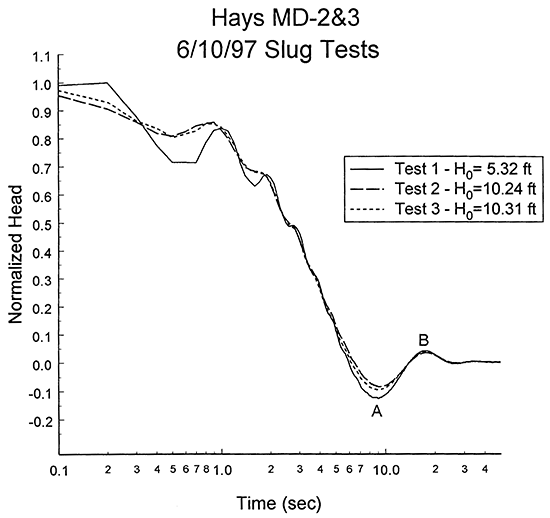
Three slug tests were performed at well MD-2&3 on June 10, 1997. Figure 4 is a plot of normalized head versus logarithm of time for this series of tests. As shown in the figure, response data from all three tests are oscillatory in nature. Although conventional theory holds that response data from repeat slug tests should coincide when graphed in a normalized format (i.e. normalized data should be independent of H0 (Butler et al., 1996)), the normalized responses plotted on Figure 4 display a dependence on H0. The most likely explanation for this dependence is that nonlinear mechanisms (Chapter 8 of Butler, 1997; McElwee and Zenner, 1998) are affecting response data. The impact of these mechanisms, however, does not appear great. Note that the absolute value of the normalized head for test one at the bottom of the first trough (point A on Figure 4) is 1.3 times greater than that of test three, while the normalized head for test one at the first peak (point B) is 1.1 times greater than that of test three. Thus, the relative difference between the normalized responses for these tests decreases significantly during the course of the tests, an indication that the influence of nonlinear mechanisms is diminishing with time. since the H0 for tests two and three differed by less than 0.1 ft, the influence of dynamic skin effects can be assessed by examining the differences between the normalized response plots for these tests. The similarity in the response plots indicates that dynamic skin effects are quite small at this well.
Figure 4--Normalized head (H(t)/H0) versus the logarithm of time since test initiation for slug tests at monitoring well MD-2&3.
Since neither the influence of nonlinear mechanisms nor that of a dynamic skin appears large, the response data were analyzed with the linearized variant of the McElwee et al. model. Figure 5 is a plot of normalized data from tests one and three, with two type curves from the linearized variant of the McElwee et al. model. Each type curve is labelled with Cd (dimensionless damping parameter) and Le (effective length of water column above the top of the screen) values. Note that little significance should be attached to differences between test responses and the type curves prior to point A because of the relatively large influence of noninstantaneous depressurization and nonlinear mechanisms in the early portions of the tests. The Cd=0.9 type curve is considered the most reasonable fit to the data for two reasons: 1) this curve seems to closely match the oscillation frequency of the test data; and 2) this curve serves as an upper bound on the absolute magnitude of the response data.
Figure 5--Normalized head (H(t)/H0) versus the logarithm of time since test initiation plot for tests one and three at monitoring well MD-2&3 with two type curves from the linearized variant of the McElwee et al. model (type curve labels defined in text).
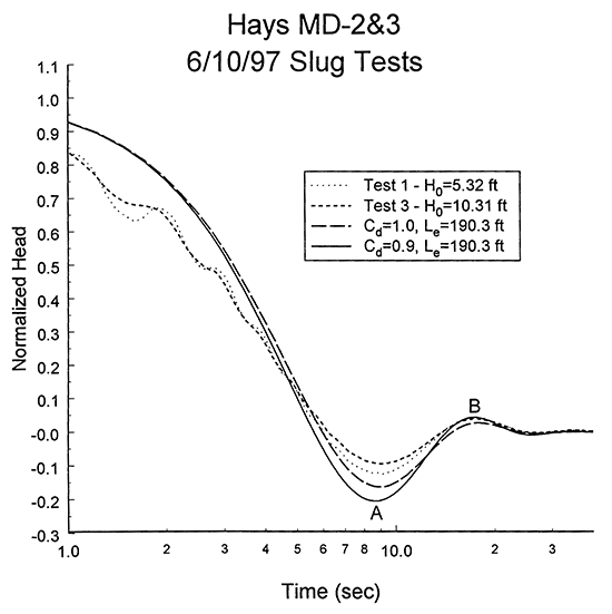
Note that the absolute magnitude of the normalized response data at point A increases with decreases in H0. Undoubtedly, this increase would have continued if tests had been initiated with smaller H0. The Cd=0.9 type curve appears to be a reasonable bound on the absolute magnitude of the normalized data for H0 approaching zero at A. This type curve also appears to be a reasonable bound on the normalized data at B. Using the Cd and Le values determined from the type curve match, the well construction information from Table 1, and the assumption of isotropy, the radial component of hydraulic conductivity can be estimated using equation (8.9c) of Butler (1997), which is designated as equation (1) for this report:
![]()
where
b = effective screen length, [L];
Cd = dimensionless damping parameter;
g = gravitational acceleration, [L2/T];
Kr = radial component of hydraulic conductivity, [L/T];
Kz = vertical component of hydraulic conductivity, [L/T];
Le = effective length of water column above the top of the
screen, [L];
rc = radius of well casing, [L];
rw = effective radius of well screen, [L];
ψ = ![]() , dimensionless.
, dimensionless.
The resulting hydraulic conductivity estimate of 12.9 ft/day should be considered a lower bound on the hydraulic conductivity of the formation in the vicinity of well MD-2&3 primarily because the nominal screen length from Table 1 was used for the effective screen length in equation (1) and the assumption of isotropy. As shown in Figure 2.4B of Butler (1997), the effective screen length is undoubtedly less than the nominal screen length as a result of incomplete well development. Although isotropy was assumed for the analysis, the sand thickness estimate given in Table 1 indicates that there is little possibility of slug-induced vertical flow outside the screened interval. For this situation, previous theoretical results, which are summarized in Figure 5.12 of Butler (1997), indicate that the assumption of isotropy could produce an underprediction in hydraulic conductivity of close to 50%. Thus, incomplete well development and little to no vertical flow outside the screened interval could easily lead to an underprediction in hydraulic conductivity of close to a factor of two. Note that at this well the nominal screen length (50 ft) and the estimated thickness of the Dakota sands (46 ft) are quite similar, so the nominal screen length was used as the effective screen length. At wells MD-1 and MD-6, however, the estimated sand thickness is much less than the nominal screen length. For those wells, the estimated sand thickness was used for the effective screen length.
The nature of the hydraulic connection between well MD-2&3 and the Dakota sands was assessed by comparing the hydraulic conductivity value determined in this analysis to values obtained at other sites in the Dakota aquifer. The hydraulic conductivity estimate of 12.9 ft/day converts to a value of 11.1 ft/day at the standard reporting temperature of 15.6 deg. C. A hydraulic conductivity estimate of 11.1 ft/day is consistent with other conductivity estimates obtained for the Dakota aquifer in Kansas (e.g., Macfarlane et al., 1990). Thus, given that this estimate is a lower bound on the hydraulic conductivity of the Dakota sands in the vicinity of well MD-2&3, the hydraulic connection between the well and the aquifer appears reasonably good.
Note that the oscillatory responses seen in all three tests at this well are usually an indication of a formation of very high hydraulic conductivity. However, a hydraulic conductivity estimate of 12.9 ft/day is over an order of magnitude below what normally would be considered "very high" hydraulic conductivity. As Ross (1985) and others have shown, oscillatory behavior can be produced in cases where the water column above the top of the screen is quite long and the formation is only of moderate hydraulic conductivity. Thus, at well MD-2&3, the oscillatory responses are considered to be primarily a product of the long column of water above the top of the screen. Note that based on the well construction information given in Table 1 and the depth to water measurement taken immediately prior to the slug tests on June 10, 1997, a value of 184.3 ft was calculated for the length of the column of water above the top of the screen. This value is within 4% of the estimate of the effective column length (Le) determined from the analysis of the response data.
Three slug tests were performed at well MD-1 on June 10, 1997. Figure 6 is a plot of normalized head versus logarithm of time for this series of tests. As shown in the figure, the response data do not display the oscillatory behavior seen in tests at all the other monitoring wells in the Hays well field. The differences seen between tests at late times are most likely a product of relatively minor dynamic skin effects and small errors in the H0 estimates. There is no indication that nonlinear mechanisms are affecting the response data.
Figure 6--Normalized head (H(t)/H0) versus the logarithm of time since test initiation plot for slug tests at monitoring well MD-1.
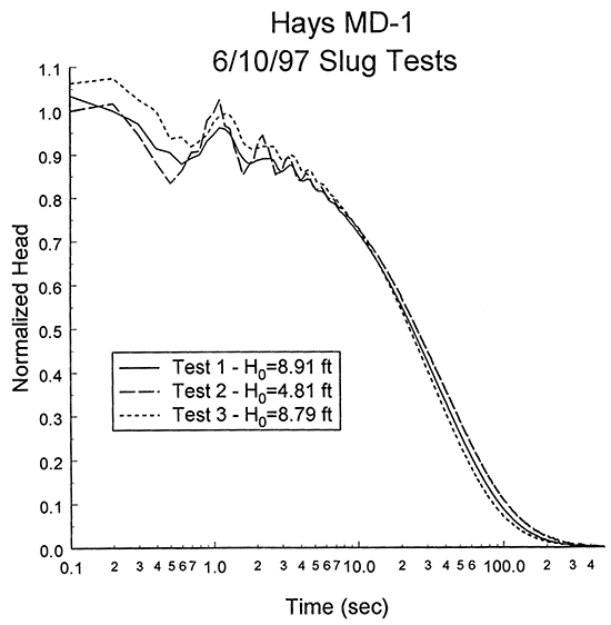
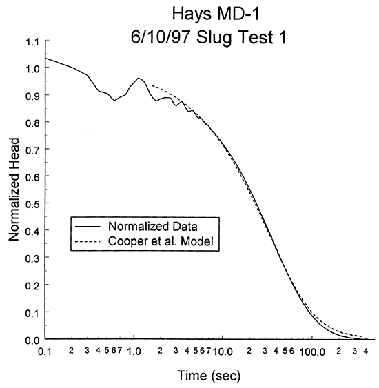
The information presented in Table 2 indicates that test one came closest to full recovery prior to depressurization and that the H0 estimates obtained from the air- and water-pressure transducers were in reasonable agreement for this test, so the response data from test one were considered the most appropriate data set to use for the estimation of hydraulic conductivity. Since tests at MD-1 do not display the oscillatory character observed at the other four monitoring wells, the data from test one were initially analyzed with the model of Cooper et al. Figure 6 indicates that the early time data were strongly impacted by the non-instantaneous depressurization of the casing, so data from the first 1.5 seconds were removed prior to the analysis. Figure 7 displays the normalized data for test one and the best-fit Cooper et al. type curve resulting from the analysis of the truncated data set. The hydraulic conductivity and specific storage estimates determined through this analysis were 1.2 ft/day and 1.3 X 10⁻⁷ ft-1, respectively. Note that a specific storage estimate of 1.3 X 10⁻⁷ ft-1 would be considered unreasonably low for the Dakota sands. As emphasized by Butler (1997), an implausibly low specific storage estimate is an indication of a low-permeability well skin or a slug test with a significant component of vertical flow (vertical flow assumed negligible in theoretical model of Cooper et al.). Since MD-1 is screened essentially through the entire interval of Dakota sands (37 ft according to the estimate given in Table 1), there is little possibility that the test induced a significant component of vertical flow. Thus, the most likely explanation for the implausibly low specific storage estimate is that there is a lowpermeability well skin at MD-1.
Figure 7--Normalized head (H(t)/H0) versus the logarithm of time since test initiation plot for test one at monitoring well MD-1 and the best-fit Cooper et al. type curve.
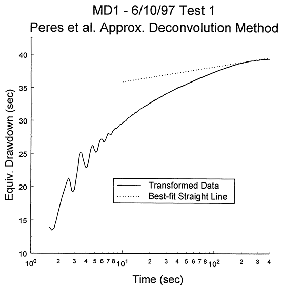
As stated in the Methodology section, the approximate deconvolution method of Peres et al. (1989) is often useful when a low-permeability well skin is affecting the response data. The data from test one at MD-1 were therefore also analyzed with this method. Figure 8 is a plot of the response data after they have been transformed into the equivalent drawdown required for the Peres et al. method. As described by Butler (1997), the concave-downward curvature of the plot is a common feature of tests performed in the presence of a low-permeability skin. The dotted line is the best-fit straight line to the equivalent drawdown between 200 and 400 seconds. Using the slope of this line and the sand thickness from Table 1, a hydraulic conductivity estimate of 3.8 ft/day is obtained. Since the equivalent drawdown plot has a distinct concave-downward curvature for the entire test period, this estimate must be considered a lower bound on the hydraulic conductivity of the Dakota sands in the vicinity of the test well. If equivalent drawdown from later time intervals could be utilized, the hydraulic conductivity estimate would undoubtedly be larger. Sensor and background noise, however, preclude later time intervals from being used for this test.
Figure 8--Equivalent drawdown versus the logarithm of time since test initiation plot for test one at monitoring well MD-1 and best-fit line for drawdown in time interval between 200 and 400 seconds.
In an ideal situation, the hydraulic conductivity of the material immediately adjacent to the well screen is the same as the bulk average conductivity of the formation. In such a situation, the various analysis methods should yield conductivity estimates that are quite similar (e.g., Chapter 5 of Butler (1997)). However, in the case of tests performed at well MD-1, the conductivity estimate obtained using the approximate deconvolution method is over a factor of three larger than that obtained with the Cooper et al. method. Given the character of these two methods, the most likely explanation for this difference is that there is a low-permeability well skin affecting test responses at MD-1.
Since the major objective of these slug tests was to assess the suitability of the monitoring wells for use as observation wells for pumping tests in the Dakota well field, the potential impact of this low-permeability well skin on drawdown measurements at MD-1 must be considered. Butler (1990) and Butler and Liu (1993) performed theoretical analyses of the impact of well skins in such situations. Given that MD-1 is 484 feet (P. Allen Macfarlane, personal communication) from D-1, the closest pumping well, and assuming that the well skin is at most 1.5 feet in radius and has a hydraulic conductivity that is one order of magnitude smaller than that of the formation, these theoretical analyses (Figure 6 of Butler (1990) and Figure 5 of Butler and Liu (1993)) indicate that the well skin will have virtually no effect on drawdown during a pumping test. Thus, although the hydraulic connection between well MD-1 and the Dakota sands is affected by the presence of a low-permeability well skin, the hydraulic connection is adequate for the purposes of pumping tests performed at well D-1 and elsewhere in the Dakota well field.
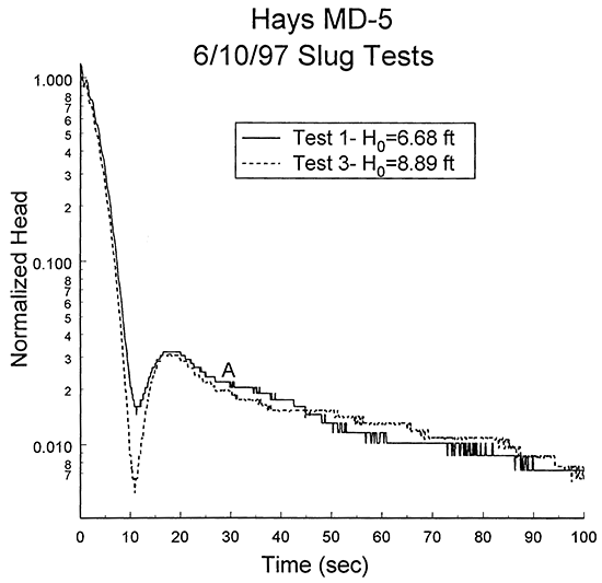
Three slug tests were performed at well MD-5 on June 10, 1997. Figure 9 is a plot of normalized head versus logarithm of time for this series of tests. As shown in the figure, response data from all three tests are slightly oscillatory in nature. Although there may be a small head dependence in the response data, the differences between the normalized responses are most probably a product of relatively minor dynamic skin effects. The most noteworthy characteristic of these tests is the "two-stage" nature of the responses. The first stage, which lasts to approximately point A on Figure 9, is oscillatory in nature, while the second stage is the classic overdamped response characteristic of slug tests in formations of moderate or lower hydraulic conductivity (see pp. 149-150 of Butler (1997)). Figure 10 is a plot of the logarithm of normalized head versus time that more clearly displays the two-stage nature of the response data.
Figure 9--Normalized head (H(t)/H0) versus the logarithm of time since test initiation plot for slug tests at monitoring well MD-5.
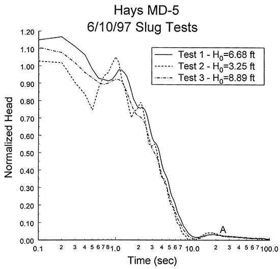
Figure 10-Logarithm of normalized head (H(t)/H0) versus the time since test initiation plot for tests one and three at monitoring well MD-5.
Response data with the two-stage character displayed in Figures 9 and 10 have apparently not previously been reported in the literature. There are several possible explanations for this phenomenon. First, it is possible that these tests were essentially over at point A and that responses after this time are simply a product of sensor drift or background trends. This explanation is considered unlikely because all three tests recovered to approximately the same head (the difference between the head at the end of test 1 and that of test 3 was 0.002 ft). Since there was no further change after this head was reached, the trend explanation can be ruled out. Second, it is possible that a dynamic skin is responsible for the observed behavior. One could envision a situation in which material is mobilized by the slug-induced disturbance and is moved in a manner such that responses in the later portion of the test are overdamped in nature. This possibili ty, however, can be ruled out on the basis of the consistency between tests. One would expect dynamic skin effects to have a large component of randomness. However, as shown most clearly in Figure 10, there is very good consistency between response data from repeat tests. A third possibility is that the behavior is somehow related to the pneumatic approach used to initiate the slug tests. However, the same equipment and procedures were used for all wells tested in the Dakota well field, so this explanation is unlikely. In addition, the transducer monitoring air pressure in the casing indicated that the air pressure in the casing returned to atmospheric pressure very quickly after casing depressurization, and remained there for the duration of each test.
The two most likely explanations are that the two-stage behavior is a product of a lateral transition in hydraulic conductivity or of a leaky annular seal. The first of these possibilities requires well MD-5 to be screened in material that is of higher conductivity than the surrounding formation. A transition to material of lower hydraulic conductivity at some distance from the well could produce the shift from oscillatory to overdamped behavior. The agreement between the normalized response data from the three tests is consistent with this explanation. Although it is possible that the hypothesized higher-conductivity zone in the vicinity of well MD-5 is a product of drilling and development, this possibility must be considered rather remote as the zone would have to be several to many meters in radius to produce the two-stage responses. Thus, if a transition in hydraulic conductivity exists, it is most likely a product of natural processes.
There have been many reports of non-oscillatory, two-stage responses in wells screened at or near the water table (e.g., Figure 6.6 of Butler (1997)). According to the hypothesis of Bouwer (1989), responses in the first stage at these wells are a product of drainage of the filter pack, while those in the second are a product of lateral flow in the formation. The leaky annular seal explanation proposed here is an extension of this theory to slug tests in highly permeable confined aquifers. According to this explanation, the screened interval is hydraulically connected to the water table as a result of an incomplete annular seal. Since the filter pack is considerably more permeable than both the Dakota sands in the vicinity of the screened interval and the shales that line the borehole above the screen, the filter pack drains relatively rapidly in response to test initiation. After the initial period of drainage is complete (approximately point A on Figure 10), the effective casing radius of the well is the radius of the borehole, modified by the porosity of the filter pack (equation (6.10) of Butler (1997)), not the nominal casing radius. In this theory, the early oscillatory behavior is a product of an initial effective casing radius equal to the nominal casing radius. The disappearance of the oscillations is caused by the transition to a larger effective casing radius. At well MD-5, the borehole radius is approximately four times larger than the nominal casing radius. A difference in radii of this size would cause over an order of magnitude increase in the dimensionless damping parameter (Cd), which, as shown in Figure 8.6 of Butler (1997), could easily produce a transition from oscillatory to overdamped conditions.
Based on the response data from well MD-5, it is difficult to determine which of these final two possibilities is the most likely explanation for the two-stage character of the responses. However, as will be discussed in the following section, similar behavior was also seen at well MD-6. In fact, the transition from oscillatory to overdamped behavior occurred at approximately the same time at both wells. Since these two wells have the same borehole and casing radii, a similar transition time would be expected in the case of an incomplete annular seal. A similar transition time would have to be considered rather serendipitous for the lateral transition hypothesis. Thus, the leaky annular seal hypothesis is considered the most likely explanation for the observed behavior.
There are currently no models to analyze data with the two-stage character displayed in Figures 9 and 10. If the lateral transition hypothesis is appropriate, the model of Kipp (1985) could be extended to consider this situation. This extension, however, has not yet been done. If the leaky annular seal hypothesis is appropriate, the model of Hvorslev (1951) could be used to fit the response data after point A on Figure 10. The absolute heads for times after point A, however, are so small (<0.15 ft) that the effects of a dynamic skin, background noise, and sensor resolution make these data of little use for analysis purposes. Thus, the analysis of the response data can only be rather qualitative in nature.
Since oscillatory behavior was observed early in the test, the linearized variant of the McElwee et al. model can be utilized to estimate a lower bound on the hydraulic conductivity of the material adjacent to the screened interval. According to this model, a Cd (dimensionless damping parameter) value of two is the transition between oscillatory (<2) and overdamped (>2) responses. Thus, since oscillatory responses were observed, a value of two would be a clear upper bound on the magnitude of Cd for these tests. Unfortunately, at the time this report was prepared, there was no WWC-5 form available for well MD-5 (P. Allen Macfarlane, personal communication). Thus, estimates for the effective screen length (80 ft) and the effective length of the water column above the top of the screen (assumed equal to the nominal length of 178 ft) were obtained from the nearby pumping well, D-5, which was most probably screened over a similar interval. The sUbstitution of the Cd estimate and the well construction parameters into equation (1) yields a hydraulic conductivity estimate of 4.1 ft/day. Given the assumptions that were adopted for this analysis (Cd=2, effective casing radius equals nominal casing radius, etc.), the conductivity of the material in the vicinity of well MD-5 is likely a factor of two to three times larger than this estimate of 4.1 ft/day. Since this estimate is a very conservative lower bound on the hydraulic conductivity of the Dakota sands in the vicinity of MD-5, the hydraulic connection between the well and the aquifer appears reasonably good.
The major objective of this program of slug tests was to assess the suitability of the monitoring wells for use as observation wells for pumping tests in the Dakota well field. Thus, the potential impact of a leaky annular seal on drawdown at MD-5 must be considered. The borehole is lined with low-conductivity materials above the screened interval, so there is little potential for significant movement of water down the borehole during a pumping test. In this case, the major effect of a leaky annulus is to increase the influence of well-bore storage (a result of the larger effective casing radius). For drawdown produced by pumping at well D-5, this effect will be quite small and limited to very early times after initiation of pumping. The impact on drawdown produced by pumping at wells other than D-5 will be negligible.
The general conclusion of this analysis of the slug tests at well MD-5 is that the well seems to be in good hydraulic connection with the Dakota sands. Although the annular seal is apparently incomplete, this condition will have little to no impact on drawdown produced by pumping in the Dakota well field.
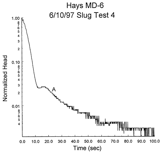
Four slug tests were performed at well MD-6 on June 10, 1997. Figure 11 is a plot of normalized head versus logarithm of time for this series of tests, while Figure 12 is the same data in a logarithm of normalized head versus time format. As shown in these figures, response data from all four tests display a two-stage character somewhat similar to that seen at well MD-5. In this case, however, test responses appear to be closer to the transition between oscillatory and overdamped behavior, as only data from test 4 (Figure 13) has a readily discernible oscillatory character. The primary feature of the early-time data from the other tests is the concave-downward curvature that Butler (1997) states is a characteristic of response data near the transition between oscillatory and overdamped responses. The similarity between the normalized responses for the first three tests indicates that dynamic skin effects can be assumed negligible at this well. The difference between the final test and the first three is most probably a reflection of a head dependence in the response data. The dependence, however, is relatively small and can be ignored for the purposes of this analysis.
Figure 11--Normalized head (H(t)/H0) versus the logarithm of time since test initiation plot for slug tests at monitoring well MD-6.
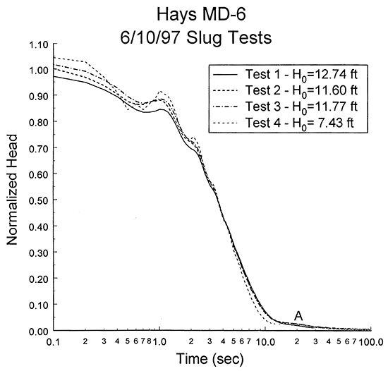
Figure 12--Logarithm of normalized head (H(t)/H0) versus the time since test initiation plot for slug tests at monitoring well MD-6.
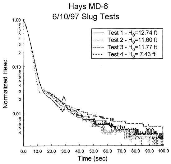
Figure 13--Logarithm of normalized head (H(t)/H0) versus the time since test initiation plot for test four at monitoring well MD-6.
The two most likely explanations for the two-stage character of the response data are, as discussed in the previous section, a lateral transition into material of lower hydraulic conductivity and a leaky annular seal. since wells MD-5 and MD-6 have the same borehole and casing radii, and response plots (cf. Figures 10 and 13) indicate a similar time for the transition from oscillatory to overdamped responses, the leaky annular seal theory is considered the most likely explanation for the observed behavior.
A lower bound on the hydraulic conductivity of the Dakota sands adjacent to the screened interval can be estimated using the same approach as in the previous section. A Cd (dimensionless damping parameter) value of two, the well construction parameters listed in Table 1, and an effective column length equal to the measured length of the water column above the top of the screen (207 ft) can be substituted into equation (1) to obtain a hydraulic conductivity estimate of 9.3 ft/day. Since the oscillatory character of the response data at MD-6 is quite weak, the dimensionless damping parameter is probably close to the assumed value of two. Thus, this conductivity estimate should be within a factor of two of the hydraulic conductivity of the material in the vicinity of the screened interval. Note that this estimate of 9.3 ft/day converts to a value of 8.0 ft/day at the standard reporting temperature of 15.6 deg. C. Given that this estimate is a lower bound on the hydraulic conductivity of the Dakota sands in the vicinity of MD-6, but yet is still consistent with other conductivity estimates obtained for the Dakota aquifer in Kansas (e.g., Macfarlane et al., 1990), the hydraulic connection between the well and the aquifer appears reasonably good.
As discussed in the previous section, the major effect of a leaky annulus is to increase the influence of well-bore storage. Since well MD-6 is approximately 261 ft (P. Allen Macfarlane, personal communication) from D-6, the nearest pumping well, the impact of well-bore storage on drawdown will be very small and limited to early times after commencement of pumping at well D-6. The impact on drawdown produced by pumping at other wells in the Dakota well field will be negligible.
The general conclusion of this analysis of the slug tests at well MD-6 is that the well seems to be in good hydraulic connection with the Dakota sands. Although the annular seal is apparently incomplete, this condition will have essentially no impact on drawdown produced by pumping in the Dakota well field.
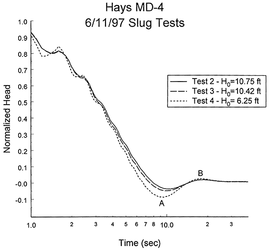
Four slug tests were performed at well MD-4 on June 11, 1997. Unfortunately, much of the data for test one was inadvertently lost as a result of a problem during the transfer of data from the datalogger to the laptop computer. Figure 14 is a plot of normalized head versus logarithm of time for the last three tests of this series. As shown in the figure, response data from all three tests were oscillatory in nature. The close agreement between responses from tests two and three indicates that dynamic skin effects were relatively minor at this well. However, the differences between those tests and test four indicate that nonlinear mechanisms are affecting the test data. The impact of these mechanisms is most pronounced in the early stages of the tests. Figure 15 is a normalized head versus logarithm of time plot that more clearly shows the differences between the tests. Note that the absolute value of the normalized head for test four at the bottom of the first trough (point A on Figure 15) is 1.8 times greater than that of test three, while the normalized head for test four at the first peak (point B) is 1.3 times greater than that of test three. An even greater decrease from A to B was seen in comparisons between tests two and four. Thus, the relative difference between the normalized responses decreases significantly with time, an indication that the influence of nonlinear mechanisms is diminishing during the course of a test.
Figure 14--Normalized head (H(t)/H0) versus the logarithm of time since test initiation plot for slug tests at monitoring well MD-4.
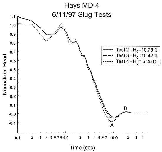
Figure 15--Normalized head (H(t)/H0) versus the logarithm of time since test initiation plot for slug tests at monitoring well MD-4.
Since the influence of nonlinear mechanisms appears to significantly decrease during the course of a test, the response data were analyzed with the linearized variant of the McElwee et al. model. Figure 16 is a plot of the normalized response data from test four, and two type curves from the linearized variant of the McElwee et al. model. Each type curve is labelled with a Cd (dimensionless damping- parameter) value. Note that independent calculations based on a method described in Chapter 8 of Butler (1997) indicated that Le (the effective length of the water column above the screen) was approximately equal to the measured length of the water column above the screen (200.8 ft) for these tests.
Figure 16--Normalized head (H(t)/H0) versus the time since test initiation plot for test four at monitoring well MD-4 with two type curves from the linearized variant of the McElwee et al. model (type curve labels defined in text).
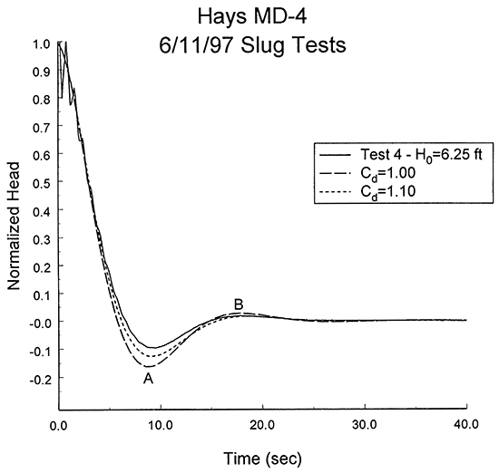
The Cd=1.00 type curve is considered the most reasonable fit to the test data because it serves as an upper bound on the absolute magnitude of the normalized responses. Figure 15 indicates that the absolute magnitude of the normalized response data at point A increases with decreases in H0. Undoubtedly, that increase would have continued if tests had been initiated with smaller H0. The Cd=1.00 type curve appears to be a reasonable bound on the absolute magnitude of the normalized response data for H0 approaching zero at A. This type curve also appears to be a reasonable bound on the normalized response data at B. Substituting Cd=1.00, Le=200.8 ft, and the well construction information from Table 1 into equation (1), and assuming isotropy in hydraulic conductivity, yields a hydraulic conductivity estimate of 8.0 ft/day. This estimate should be considered a lower bound on the hydraulic conductivity of the Dakota sands in the vicinity of well MD-4 because the nominal screen length is undoubtedly greater than the effective screen length. Since the estimated sand thickness is greater than the nominal screen length, there is the possibility of slug-induced vertical flow outside of the screened interval during these tests. Thus, the assumption of isotropy should not be the source of a significant underprediction in hydraulic conductivity at well MD-4.
The nature of the hydraulic connection between well MD-4 and the Dakota sands was assessed by comparing the hydraulic conductivity estimate with values obtained from elsewhere in the Dakota aquifer. The hydraulic conductivity estimate of 8.0 ft/day converts to a value of 6.9 ft/day at the standard reporting temperature of 15.6 deg. C. This value of 6.9 ft/day is consistent with other conductivity estimates obtained for the Dakota aquifer in Kansas (e.g., Macfarlane et al., 1990). Thus, given that this estimate is a lower bound on the hydraulic conductivity of the Dakota sands in the vicinity of MD-4, the hydraulic connection between the well and the aquifer appears reasonably good.
A series of slug tests were performed by the Kansas Geological Survey in the monitoring wells in the Dakota well field of the city of Hays in Ellis County, Kansas in June of 1997. These tests were designed to assess the suitability of the monitoring wells for use as observation wells for pumping tests performed in the Dakota well field. Table 3 provides a summary of the results of the test program. In all cases, the evaluation of monitoring-well suitability was based on a comparison of the estimates of hydraulic conductivity listed in Table 3 with that expected for the Dakota sands in the vicinity of the Hays well field. Based on this comparison, four of the five wells appear to be in reasonable hydraulic connection with the Dakota sands. The hydraulic connection at well MD-1 appears to be affected by a lowpermeability well skin. This skin, however, will have little to no impact on drawdown during a pumping test in the Dakota well field. Al though analyses of response data from wells MD-5 and MD-6 indicate that tests at those wells may be affected by leaky annular seals, this will have little to no impact on drawdown during a pumping test in the Dakota well field. Thus, the general conclusion of the June 1997 test program is that all five monitoring wells are suitable for use as observation wells for pumping tests performed in the Dakota well field of the city of Hays.
Table 3--Summary of results of June 1997 slug tests in the Dakota well field of the city of Hays
| Test Well | Hydraulic Conductivity Estimate (ft/d)1 |
Hydraulic Connection2 |
|---|---|---|
| MD-1 | > 3.83 (3.3) | incomplete4 |
| MD-2&3 | > 12.9 (11.1) | reasonable |
| MD-4 | > 8.0 (6.9) | reasonable |
| MD-5 | > 4.15 (3.5) | reasonable |
| MD-6 | > 9.35 (8.0) | reasonable |
| 1 - in general, estimates should be considered lower bounds on the hydraulic conductivity of the Dakota sands because of uncertainty regarding the effective screen length and the degree of anisotropy; values for standard reporting conditions (Fetter, 1994) are given in parentheses 2 - refers to hydraulic connection between the well and the Dakota sands 3 - data at this well have clearly been affected by a low-K well skin, so hydraulic conductivity of the Dakota sands may be considerably greater than listed value 4 - low-K well skin affecting hydraulic connection 5 - response data indicate that leaky annular seals may have affected tests at these wells. Since there are no theoretical slug-test models that incorporate water movement in an incompletely sealed annulus, these tests were analyzed with an approximate approach that provides conservative lower bounds on the hydraulic conductivity of the Dakota sands. |
||
Bohling, G. C., C. D. McElwee, J. J. Butler, Jr., and W. Z. Liu, 1990, User's Guide to Well Test Design and Analysis with SUPRPUMP version 1.0: Kansas Geological Survey, Computer Program Series 90-3, 95 pp.
Bohling, G. C., and C. D. McElwee, 1992, SUPRPUMP: An interactive program for well test analysis and design, Ground Water, v. 30, no. 2, pp. 262-268.
Bouwer, H., 1989, The Bouwer and Rice slug test--an update: Ground Water, v. 27, no. 3, pp. 304-309.
Butler, J. J., Jr., 1990, The role of pumping tests in site characterization: Some theoretical considerations: Ground Water, v. 28, no. 3, pp. 394-402.
Butler, J. J., Jr., 1997, The Design, Performance, and Analysis of Slug Tests: Lewis Pub., Boca Raton, 252 pp.
Butler, J. J., Jr., and J. M. Healey, 1998, Relationship between pumping-test and slug-test parameters: Scale effect or artifact?: Ground Water, v. 36, no. 2, pp. 305-313.
Butler, J. J., Jr., and W. Z. Liu, 1993, Pumping tests in nonuniform aquifers: The radially asymmetric case: Water Resources Research, v. 29, no. 2, pp. 259-269.
Butler, J. J., Jr., C. D. McElwee, and W.Z. Liu, 1996, Improving the quality of parameter estimates obtained from slug tests: Ground Water, v. 34, no. 3, pp. 480-490.
Cooper, H.H., J. D. Bredehoeft, and I. S. Papadopulos, 1967, Response of a finite-diameter well to an instantaneous charge of water: Water Resources Research, v. 3, no. 1, pp. 263-269.
Fetter, C.W., 1994, Applied Hydrogeology: Macmillan, New York, 691 pp.
Hvorslev, M. J., 1951, Time lag and soil permeability in ground-water observations: U.S. Army Corps of Engrs. Waterways Exper. Sta. Bull no. 36, 50 pp.
Kipp, K. L., Jr., 1985, Type curve analysis of inertial effects in the response of a well to a slug test: Water Resources Research, v. 21, no. 9, pp. 1397-1408.
Kruseman, G. P. and N. A. de Ridder, 1990, Analysis and Evaluation of Pumping Test Data: ILRI Publication 47, ILRI, The Netherlands, 377 pp.
Macfarlane, P. A., D. O. Whittemore, M. A. Townsend, J. H. Doveton, V. J. Hamilton, W. G. Coyle, III, A. Wade, G. L. Macpherson, and R. D. Black, 1990, The Dakota Aquifer Program: Annual report, FY89: Kansas Geological Survey, Open-File Rept. 90-27, 302 pp. [available online]
MathSoft, Inc., 1996, Axum User's Guide: 370 pp.
MathSoft, Inc., 1997, Mathcad 7.0 User's Guide: 684 pp.
McElwee, C. D., G.C. Bohling, and J.J. Butler, Jr., 1995, Sensitivity analysis of slug tests, I. The slugged well: Jour. of Hydrology, v. 164, pp. 53-67.
McElwee, C.D., and M.A. Zenner, 1998, A nonlinear model for analysis of slug-test data: Water Resources Research, v. 34, no. 1, pp. 55-66.
Peres, A. M. M., M. Onur, and A. C. Reynolds, 1989, A new analysis procedure for determining aquifer properties from slug test data: Water Resources Research, v. 25, no. 7, pp. 1591-1602.
Ross, B., 1985, Theory of the oscillating slug test in deep wells; in, Memoirs of the 17th Intern. Cong. on the Hydrogeology of Rocks of Low Permeability: v. 17, pt. 2, International Assoc. of Hydrogeologists, pp. 44-51.
Spane, F. A., Jr., and S. K. Wurstner, 1993, DERIV: A program for calculating pressure derivatives for use in hydraulic test analysis, Ground Water, v. 31, no. 5, pp. 814-822.
Weast, R. C. (ed.), 1976, CRC Handbook of Chemistry and Physics: CRC Press, Cleveland, OH, pp. D252-D253.
Kansas Geological Survey, Geohydrology
Placed online Feb. 27, 2015
Comments to webadmin@kgs.ku.edu
The URL for this page is http://www.kgs.ku.edu/Hydro/Publications/1998/OFR98_15B/index.html