Kansas Geological Survey, Open-file Report 96-1d
KGS Open File Report 96-1d
Released 1996
To read this report, you will need the Acrobat PDF Reader, available free from Adobe.
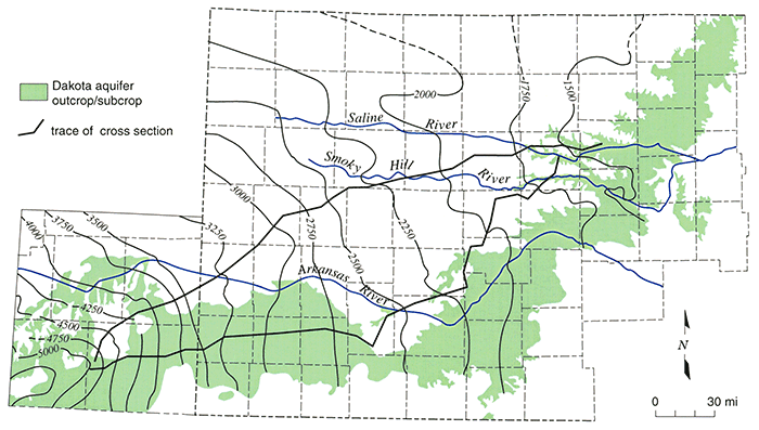
Beginning in FY92, work began to integrate the findings of the subregional investigations of the Dakota aquifer where it is presently undergoing development. Within this region there is adequate subsurface geologic and hydrologic information to characterize the regional hydrogeology of the Dakota in some detail. The underlying goal of this effort was to understand primary influences on the steady-state flow system in the Dakota in Kansas. It was felt that the results of this work could serve as a basis for later efforts to develop realistic management alternatives for using the Dakota as a water supply, including the use of management models. The research proceeded using two approaches in parallel. In the first, two-dimensional vertical profile models of the regional hydrogeology of the upper of the regional flow system were developed along two transect lines extending from the regional recharge area in southeastern Colorado to the regional discharge area in central Kansas (Figure 1). The purpose of this work was to examine hydrologic relationships between the various hydrostratigraphic units and the influence of topography on the flow system hierarchy in an exploratory fashion. The modeling results of the northern transect were reported in the FY92 Annual Report and the results of subsequent work using geochemical tracers along this traverse were reported in the FY93 Annual Report. Following this, work began on the southern traverse the subject of this report. In the other approach, a three-dimensional, steady-state regional flow model of the Dakota aquifer in southeastern Colorado and Kansas was assembled and calibrated to develop further conceptual understandings of the regional flow system, including the Dakota aquifer. The model assembly was described in the FY93 Annual Report. The results from the modeling efforts along the southern traverse and the calibration and discussion of the results from the regional modeling are reported in the FY94 Annual Report.
Figure 1--Traces of the northern and southern vertical profiles extending from southeastern Colorado into central Kansas.
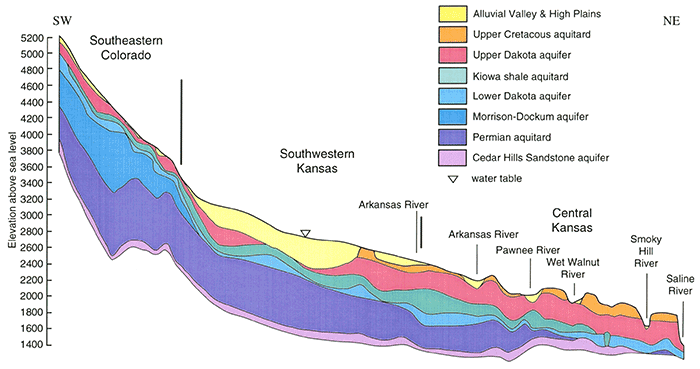
Southeastern Colorado and southwestern and central Kansas are located in the Raton Section, Colorado Piedmont, High Plains, and Plains Border sections of the Great Plains physiographic province (Fenneman, 1946). The land surface slopes to the east and decreases in elevation from approximately 5,000 ft (1,524 m) in southeastern Colorado to 1,400 ft (427 m) in central Kansas (Figure 2). Both traverses extend across the Arkansas, Smoky Hill, and Saline River drainage basins. The valleys cut by these river systems into unconsolidated Cenozoic deposits and Cretaceous bedrock locally increase the topographic relief significantly in central Kansas.
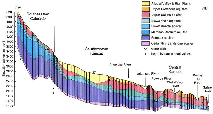
Figure 2--Aquifer and aquitard units in the southern vertical profile model.
The climate of the region is warm, continental semiarid in all except the eastern portions of the study area in central Kansas, where the climate is subhumid continental (Dugan and Peckenpaugh, 1985). The mean annual temperature is approximately 54°F (12.2 °C) across the study area. Mean annual rainfall for the period 1951-1980 ranged from 15 in (38.1 cm) in southeastern Colorado to 28.5 in (72.4 cm) in central Kansas. Approximately 75% of the precipitation falls mainly during the warm season months of the year. Because of the low relative humidity, high average wind velocities, and abundant sunshine, the potential evaporation exceeds the average annual precipitation over most of the region. Dugan and Peckenpaugh (1985) calculated that the potential mean annual recharge to ground water from precipitation ranges from less than 0.1 in (0.2 cm) in southeastern Colorado to 1-2 in (2.5-5.0 cm) in central Kansas.
The regional stratigraphy and hydrostratigraphy are summarized in Table 1 and shown along the transect in Figure 2. The methodology used to define regional hydro stratigraphic units is discussed in detail by Macfarlane et al. (1992) and Macfarlane (1993). The hydrostratigraphy consists of six major aquifers and three aquitards.
Table 1--Hydrostratigraphy and model layers in the southern vertical profile model.
| Era | System | Rock Stratigraphic Units |
Hydrostratigraphic Units |
Model Layer | |
|---|---|---|---|---|---|
| Cenozoic | Quaternary | Unconsolidated alluvial and eolian deposits |
Alluvial Valley & High Plains aquifers |
1 | |
| Tertiary | Ogallala Formation | ||||
| Mesozoic | Cretaceous | Colorado Group |
Pierre Shale | Upper Cretaceous aquitard | 2 |
| Niobrara Chalk | |||||
| Carlile Shale | |||||
| Greenhorn Limestone | |||||
| Graneros Shale | |||||
| Dakota Formation |
Jansen Member | Upper Dakota aquifer | 3 | ||
| Terra Cotta Member | |||||
| Kiowa Formation |
Kiowa shale aquitard | 4 | |||
| Longford Member | Lower Dakota aquifer | 5 | |||
| Cheyenne Sandstone | |||||
| Triassic/ Jurassic |
Dockum Group/ Morrison Formation |
Morrison-Dockum aquifer | 6 | ||
| Paleozoic | Permian | Undifferentiated Permian | Permian aquitard | 7 | |
| Cedar Hills Sandstone | Cedar Hills Sandstone aquifer | 8 | |||
Two distinct ground-water flow "corridors" can be distinguished from the Dakota aquifer predevelopment potentiometric surface map (Figure 1). The northern flow "corridor" begins in eastern Las Animas County and extends northeastward across the Arkansas River into west-central and northwestern Kansas and turns eastward into central Kansas. The southern flow "corridor" begins in eastern Las Animas County and extends eastward into southwestern Kansas and then turns northeastward toward central Kansas. The potentiometric-surface map suggests that the primary recharge area for the Dakota aquifer in Kansas is in southeastern Las Animas and western Baca counties in Colorado on the Sierra Grande uplift. In this area the Dakota aquifer is at the surface and is recharged directly by infiltrating precipitation. The primary ground-water discharge area appears to be in central Kansas where the major drainages, such as the Smoky Hill and Saline Rivers, cross the outcrop of the Dakota aquifer. The 1,500-ft (460-m) head contour suggests that ground-water flow is focused in this part of the outcrop zone (see Figure 1). In this area salt springs, seeps, and marshes are a common occurrence (Macfarlane et al., 1990). The northern and southern vertical profile models are parallel to flow lines in the northern and southern flow "corridors", respectively.
Previous investigations have established the preeminence of the Upper Cretaceous aquitard as a major factor that exerts control on the flow system in the central Great Plains (Helgesen et al., 1993; Belitz, 1985; Belitz and Bredehoeft, 1988; Leonard et al., 1983; Helgesen et al., 1982). In the work on the northern traverse, much of the attention was focused on the influence of the Upper Cretaceous aquitard on the upper Dakota aquifer. The upper Dakota aquifer was considered important to the regional flow system because it is hydraulically continuous across the vertical profile and is more transmissive than the other shallow aquifers below the thick aquitard. The modeling results confirmed that the upper Dakota acts as a drain beneath the aquitard (Macfarlane, 1993). However, the water budget showed that most of the flow cycling through the flow system is tied up in local flow systems in southeastern Colorado and central Kansas where the Upper Cretaceous has been breached or removed by erosion. This is a consequence of the thick, low permeability aquitard overlying the Dakota and the low local topographic relief of western Kansas. As a result, it appears that very little of the flow moves from the regional recharge area in southeastern Colorado to the regional discharge area in central Kansas.
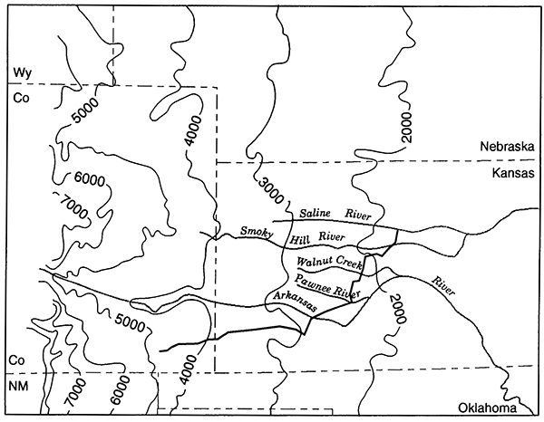
The trace of the southern vertical profile extends eastward across Baca County in southeastern Colorado and Stanton, Grant, Haskell and Gray counties in southwestern Kansas to the south of the Arkansas River (Figure 3). In southern Gray County, the trace of the vertical section turns northeastward and extends along the western edge of the outcrop!subcrop belt of the Dakota aquifer to the Saline River in central Kansas. This leg is located in Gray, Ford, Edwards, Pawnee, Rush, Barton, and Russell counties. The trace of the southern vertical profile crosses the Arkansas River in Gray County, the Pawnee River in Pawnee County, the Wet Walnut Creek in Rush County, and the Smoky Hill and Saline Rivers in Russell County. Along the southern traverse, the regional land-surface slope ranges from 38.5 ft/mi (7.3 m/km) in southeastern Colorado to 8.7 ft/mi (1.65 m/km) in southwestern and central Kansas (Figure 2). Local topographic relief is generally subdued along the southeastern Colorado and southwestern Kansas sections but is much more pronounced in the central Kansas section north of the Arkansas River crossing in Ford County. For example, in the Saline River valley of central Kansas the local topographic relief commonly exceeds 200 ft/mi (37.9 m/km).
Figure 3--Generalized land-surface topography and the major streams traversed by the vertical profile in eastern Colorado and western and central Kansas and adjacent areas.
In the subsurface, the upper Dakota is a shallow aquifer or is hydraulically connected to an overlying water-table aquifer (Figure 2). In parts of the Bear Creek drainage of Baca County, Colorado, and adjacent western Stanton County, Kansas, the upper Dakota is a near-surface aquifer overlain by a thin veneer of unsaturated unconsolidated deposits (McLaughlin, 1954; Hershey and Hampton, 1974; Latta, 1941; and Stullken and Pabst, 1982) or thinly saturated High Plains aquifer. In the Bear Creek drainage, the Dakota aquifer crops out in the stream bank and some of its tributaries. In southwest Kansas, pre-Ogallala erosion has removed the units that constitute the Upper Cretaceous aquitard and portions or all of the upper Dakota aquifer. To the east in central Kansas, late Cenozoic erosion has removed the Ogallala Formation and portions or all of the Upper Cretaceous aquitard and produced an entrenched drainage network. Consequently, the total thickness of the Upper Cretaceous aquitard only exceeds 100 ft near the Saline and Smoky Hill Rivers in Rush, Barton, and Russell counties.
It is hypothesized that in this part of Kansas the primary influence on the upper part of the regional, steady-state flow system is land-surface topography and only secondarily, the vertical hydraulic conductivity of the Upper Cretaceous aquitard. Along the trace of the southern vertical profile, the Upper Cretaceous aquitard is thin and relatively permeable due to erosional unloading of the shales. Erosion of the aquitard and entrenchment of the drainage network has brought the deeper aquifers of northwest Kansas, including the Dakota, into closer proximity to the near-surface hydrologic environment. The development of significant local topographic relief on a regionally sloping land surface produces subdivisions of the steady-state regional flow system into smaller subsystems (Toth, 1962, 1963; Freeze and Witherspoon, 1967). The greater the topographic slope, the greater the definition of a regional flow system. The greater the local topographic relief, the more well developed and vertically extensive are the local flow systems.
In the regional recharge area of southeastern Colorado, the Dakota is at the surface and is readily recharged by infiltrating precipitation. The high regional topographic slope and the moderate to low relief of the land surface favor development of shallow local flow systems superimposed on the regional flow system in the recharge area. In southwestern Kansas, the Dakota and the overlying High Plains aquifer should be a hydraulically-connected system because they are not separated by the Upper Cretaceous aquitard. However, local flow systems are not very well developed because of the low local topographic relief in these areas.
In central Kansas however, the Upper Cretaceous aquitard has been breached in the vicinity of stream valleys and the Dakota crops out at the surface or subcrops beneath unconsolidated alluvial deposits. The local topographic relief is pronounced in the vicinity of the stream valleys relative to the very low regional slope. Thus, the flow system may be dominated a series of laterally-adjacent local flow systems.
A major consequence of these developments for the Dakota aquifer is the high rate of recharge from infiltrated precipitation relative to the deeper confined aquifer of the northern vertical profile. Local flow-system development in central Kansas suggests higher rates of flow and much shorter ground-water residence times due to the short flow path lengths. As a result, there should be a greater rate of flushing of salts from the aquifer and the ground water chemistry should be more like that of the infiltrating precipitation.
Two of the primary uses of computer simulation in hydrogeology are (1) to evaluate conceptualizations of ground-water flow system dynamics and (2) to make inferences on system dynamics based on these conceptualizations. Anderson and Woessner (1992) refer to these uses collectively as the interpretive application of computer simulation. A vertical profile model of ground-water flow in the upper part of the regional flow system in southeastern Colorado and western and central Kansas is the basis for testing the hypothesis outlined here.
A significant drawback to the formulation of a fully calibrated model of the flow system is that the available hydrologic properties and head data are sparse along the trace of the vertical profile even though they are sufficient for regional characterization. Also, most of the data come from the upper Dakota and other shallow aquifers and from much deeper hydrocarbon reservoirs in Permian and Pennsylvanian rocks. Because of this, the nature of the flow system can only be inferred, and hence there is insufficient information by which to fully calibrate the model. This is acceptable because a fully calibrated model is not required when the purpose of the simulation is interpretive and not predictive (Anderson and Woessner, 1992).
Accordingly, the objectives here are to (1) describe the construction of a vertical profile model of the upper part of the flow system, (2) discuss the flow patterns in the partially calibrated steady-state model and its associated water budget, (3) to present the results of sensitivity analyses that show the effect of the hydrostratigraphy and the river valleys on the flow system, and (4) to make comparisons between the different views of the regional flow system shown in the northern and southern vertical profiles.
Computer simulation of the upper part of the regional flow system was a three-stage process, which included model design, derivation of hydraulic properties, and sensitivity analysis of the resultant partially calibrated model. Model design involved discretization of the vertical profile that encompasses the flow system and setting the boundary and initial conditions and the initial hydraulic parameter estimates for each of the hydro stratigraphic units. In the second stage the steady-state model was treated as an inverse problem. The model was used to estimate the vertical hydraulic conductivity of the aquitards and the transmissivity of the aquifers using known hydraulic head and flow rate information. Finally, sensitivity analysis was applied to the partially calibrated model developed in the second stage to determine the major influences on the flow system.
The governing equation that describes the flow of ground water in a vertical profile parallel to the flow direction is (Anderson and Woessner, 1992)
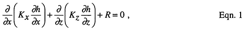
where R is a source/sink term and Kx and Kz are the x and z components of hydraulic conductivity. Eqn. 1 describes ground-water flow through a heterogeneous and anisotropic porous medium where the principal axes of hydraulic conductivity are aligned with the orthogonal x and z coordinate system axes. Sources of recharge to and discharge from the model are not indicated explicitly because they are handled separately as part of the boundary conditions, which are discussed later.
MODFLOW (McDonald and Harbaugh, 1988) was used to solve Eq. 1 along with its attendant boundary and initial conditions in the vertical profile. This software package uses a block-centered finite-difference code to simulate ground-water flow in two or three dimensions. MODFLOW was selected for this application because it can be readily adapted to a vertical profile model (Anderson and Woessner, 1992).
The model grid consists of 9 layers, 1 row, and 95 columns (Figure 4). Each model cell has a row length of 1 ft and a variable column length along the profile (the x-axis in Figure 4) from 5,709 ft to 28,546 ft. This variable cell length in the x-axis direction is used to more accurately simulate the upper water-table boundary in regions of significant topographic relief. The total length of the vertical profile from southeastern Colorado to central Kansas is 335.2 mi (539.5 km). Like the northern vertical profile, the model grid for the southern vertical profile was subdivided into three major sections on the basis of relative local and regional topographic relief in vertical profile view (Figure 4). The southeastern Colorado upland section extends from the western end of the model to the change in regional topographic slope in column 19. In this part of the model the regional topographic slope is steep and the local topographic relief is low. The southwestern Kansas section of the model extends from column 20-50, near the Arkansas River in Edwards County. This part of the model is characterized by a moderate regional topographic slope and low local relief. The central Kansas model segment (columns 51-95) the regional topographic slope is low and the local topographic relief is high due to the incised river valleys that intersect the vertical profile.
Figure 4--The vertical profile model grid consists of 8 layers, 1 row, and 95 columns of cells. The length of each cell in the column direction (along the x axis) is variable and ranges from 5,709 ft (1740 m) to 28,546 ft (8701 m). The length of each cell in the row direction (along the y axis) is 1 ft (0.3 m). The vertical exageration is 217.6X. The location of the vertical profile is shown in Figures 1 and 3. Also shown in the vertical profile are the locations of the target hydraulic data used to assess the progress of model calibration and flow-system sensitivity.
Each of the model layers represents a hydro stratigraphic unit (Table 1). The model grid and the input parameters were designed to reflect changes in the hydrostratigraphy in the vertical profile caused by the pinching out of model layers. This happens to several of the layers in the model (Figure 4). The pinchout of layers is taken into account where it occurs by continuing the layer across the model as a phantom with a transmissivity and a layer thickness of zero. Vertical hydraulic continuity is maintained where the layer is not present by assigning the same vertical conductance to the cells in the phantom layer that is assigned to cells in the overlying real layer. The vertical conductance of each cell in the real layer above was calculated by assuming that both real layers are in physical contact. Selection of initial parameter values, shown in Table 2, was guided by data collected from the literature and from unpublished sources (Macfarlane, 1993).
Table 2--Input hydraulic conductivity data for the hydrostratigraphic units in the vertical profile.
| Hydrostratigraphic Unit |
Horizontal Hydraulic Conductivity (ft/day) |
Vertical Hydraulic Conductivity (ft/day) |
|---|---|---|
| High Plains aquifer | 80 | 8.0 |
| Alluvial valley aquifers | 80 | 8 |
| Upper Cretaceous aquitard | 3.0 x 10⁻⁴ | 3.0 x 10⁻⁵ |
| Upper Dakota aquifer | 4-20 | 3.1 x 10⁻³ |
| Kiowa shale aquitard | 1.3 x 10⁻⁵ | 1.3 x 10⁻⁶ |
| Lower Dakota aquifer | 2.0 | 3.7 x 10⁻³ |
| Morrison-Dockum aquifer | 0.5 | 0.05 |
| Permian-Pennsylvanian aquitard (Layers 7 and 9) |
2.7 x 10⁻³ - 2.7 x 10⁻⁵ | 2.7 x 10⁻⁴ - 2.7 x 10⁻⁶ |
| Permian sandstone aquifer | 1.6 | 0.16 |
The boundary conditions define the hydraulic conditions on the perimeter of the model and are necessary to produce a unique solution to the flow equation (Anderson and Woessner, 1992). In the vertical profile model specified-head and no-flow boundary conditions were imposed on the perimeter. The upper model boundary represents the water table and is considered a specified-head boundary (see Figure 4). At this boundary temporal fluctuations in head are small relative to the total head difference on the water table across the model (3,560 ft) and the maximum vertical extent of the model (up to 1,700 ft). The specified-head boundary condition was applied instead of a flux boundary to minimize the number of parameters that needed adjusting during calibration. The specified-head condition allows a flux of water (recharge or discharge) to cross the water table during model execution to maintain the constant head in each cell.
Specified-head boundary conditions were also applied at two sites where there are time-invariant, vertical hydraulic head gradients that are not significant relative to the scale of the regional model. The western boundary in southeastern Colorado corresponds to the 5,179 ft (1579 m) equipotential, which is assumed to be vertical in the profile (Figure 4). Due to the limited amount of hydraulic head information available, placement of this boundary was guided by the results of modeling experiments discussed by Macfarlane (1993). The eastern boundary in central Kansas corresponds to an assumed, vertical head difference of 2 ft between the upper and lower Dakota aquifers beneath the Saline River drainage. It is assumed that the model terminates beneath the discharge area of a local flow system. The small head difference allows for the discharge of ground water from the local flow system into the stream.
A no-flow boundary was used along the bottom of the model to simulate the horizontal flow line that approximates the boundary separating the shallow upper part of the regional flow system from the lower part of the regional system (Figure 4). This flow line was drawn on the basis of modeling results described by Macfarlane (1993).
Calibration of ground-water flow models usually consists of adjusting the input parameters until a satisfactory match is achieved between the observed and the simulated hydraulic heads, fluxes, or other calibration targets (Wang and Anderson, 1982). In this research a fully calibrated model of the flow system was deemed inappropriate because of the lack of head data for many of the layers below the upper Dakota aquifer. Calibration was carried out manually by trial-and-error adjustment of the hydraulic conductivity input data to match input hydraulic head measurements. Because most of the head data were primarily from the High Plains, alluvial valley, and upper Dakota aquifers, little adjustment was made in the hydraulic parameters of layers below the upper Dakota aquifer. All the adjustments made in the values of these parameters were guided by the sensitivity analyses. Twenty-two target head values were available to check the progress of calibration (Figure 4). Of this total, 18 were in either the upper or the lower Dakota aquifers.
The results of each round of calibration were evaluated by computing the root mean square (RMS) error (Anderson and Woessner, 1992):
![]()
where hm and hs are the measured and simulated heads, respectively. This criterion was chosen because the RMS error is thought to be the best measure of uncertainty if the errors are normally distributed (Anderson and Woessner, 1992). The RMS error was also used to evaluate model sensitivity to systematic changes in layer hydraulic conductivity and boundary conditions. Initially, the steady-state model was to be considered partially calibrated when the RMS error was less than 50 ft, which is 1.3% of the total head decline (3,711 ft) across the model. This value of the RMS error is also within the probable error of many of the calibration target heads. The RMS error of the partially calibrated model is 59.9 ft, which is higher than the desired value. However, the RMS error considering only the heads in the upper and lower Dakota aquifers is 44.1 ft.
Table 3 lists the horizontal and vertical hydraulic conductivities from the partial calibration of the model. The range of horizontal hydraulic conductivities for the upper Dakota aquifer is 4-30 ft/day. The highest values are located from just north of the Pawnee River to just north of Walnut Creek. The lowest values are in southeastern Colorado and southwestern Kansas.
Table 3--Variation in layer hydraulic conductivity for the hydrostratigraphic units in the vertical profile model of the upper part of the regional flow system along the southern traverse.
| Hydrostratigraphic Unit |
Horizontal Hydraulic Conductivity (ft/day) |
Vertical Hydraulic Conductivity (ft/day) |
|---|---|---|
| High Plains aquifer | 80 | 8.0-0.8 |
| Alluvial valley aquifers | 80 | 8.0 |
| Upper Cretaceous aquitard | 3.0 x 10⁻⁴ | 9.0 x 10⁻⁵ - 4.6 x 10⁻⁷ |
| Upper Dakota aquifer | 4-30 | 3.1 x 10⁻² - 3.1 x 10⁻³ |
| Kiowa shale aquitard | 1.3 x 10⁻⁵ | 1.3 x 10⁻⁶ |
| Lower Dakota aquifer | 0.2-3.0 | 3.1 x 10⁻³ |
| Morrison-Dockum aquifer | 0.5 | 0.05 |
| Permian-Pennsylvanian aquitard (Layers 7 and 9) |
2.7 x 10⁻³ - 2.7 x 10⁻⁵ | 3.2 x 10⁻⁶ - 2.7 x 10⁻⁷ |
| Permian sandstone aquifer | 1.6 - 5.0 x 10⁻⁴ | 0.16 |
The head distribution in the partially calibrated model of the steady-state flow system is indicated by the pattern of the equipotentials shown in Figure 5. A plot showing the distribution of recharge and discharge across the upper model boundary was prepared to gain further insight into the behavior of the flow system (Figure 6). The cell-by-cell flow rates within the aquifer units were computed by MODFLOW for the constant-head cells. The positive and negative values for each node represent the net recharge and discharge, respectively, through each of the cells along the upper boundary. Not considered in this calculation is the flow of water between adjacent constant head cells. Thus the model only calculates flow vertically into or out of the model. For the other cells in the model, ZONEBUDGET (Harbaugh, 1990) was used to calculate cell-by-cell water budgets.
Figure 5--Steady-state head distribution in the partially calibrated vertical profile model. Ground-water flow is from regions of higher to regions of lower hydraulic head.
Figure 6--Recharge and discharge across the upper boundary of the southern vertical profile model. Positive fluxes indicate recharge and negative fluxes indicate discharge.
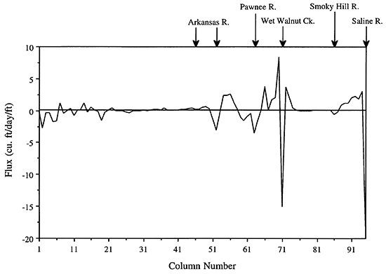
In southeastern Colorado and adjacent parts of southwestern Kansas, the equipotentials are vertical in orientation and closely spaced together (Figure 5). The steep head gradient at this end of the model is controlled by the nature of the boundary conditions: the high regional slope of the water table, the low local relief, and the specified head at the upgradient end of the model. Figure 6 shows an alternation of recharge and discharge across the upper model boundary in this section. The low-amplitude alternation of recharge and discharge suggests shallow laterally adjacent local flow systems superimposed on a regional flow system in this part of the vertical profile.
To the east in Figure 5, where the High Plains aquifer thickens, the regional gradient on the water table flattens. Recharge to and discharge from the model is relatively insignificant due to the low slope of the water table (Figure 6). The equipotentials indicate discharge of ground water from the upper Dakota to the High Plains aquifer where the Dakota has been removed by erosion. To the east the model shows the High Plains recharges the Dakota in Gray county. This clearly indicates that the Dakota and the High Plains aquifers behave as a single hydraulically connected system at steady state. In the underlying lower Dakota, the vertical flow direction is upward across the Kiowa shale aquitard to the High Plains aquifer where the upper Dakota is not present. Where the Upper Cretaceous aquitard is present in Gray and western Ford counties and south of the Arkansas River, the bending of the equipotentials suggests that recharge to the upper Dakota is somewhat restricted. Farther along the vertical profile in the area between the Arkansas River crossing in Ford County and Edwards County (Figures 1, and 5), the volumetric flux out of the model increases near the valley. This suggests that there may have been a local natural discharge area from the High Plains aquifer near Kinsley in pre-development times.
Beyond this part of the model, the local topographic relief begins to increase significantly while the regional slope of the water table appears to be maintained (Figure 5). The alternation of recharge and discharge in Figure 6 and the slight bending of the equipotentials in Figure 5 toward stream channels suggests the development local flow systems. The model indicates that the Wet Walnut and the Saline River receive significant amounts of baseflow from the upper Dakota aquifer. However, much less is discharged to the Pawnee River (about 30% of the discharge to the Saline River) and the Smoky Hill River (about 5% of the discharge to the Saline River). The very small discharge from the flow system to the Smoky Hill River is probably due to the boundary conditions. Figure 5 shows that the Smoky Hill River valley is at a higher elevation in the vertical profile than is the Saline River valley. The lower relief from the drainage divide to the valley bottom suggests that the local flow system in the Smoky Hill does not extend does not extend as deeply into the subsurface as the local flow system in the Saline (Toth, 1963) and hence will be able to capture as much of the deeper more saline ground-water flow in the Cedar Hills Sandstone aquifer.
The fixed hydraulic head gradient across the upper and lower Dakota aquifers at the eastern boundary of the model may be significantly underestimated. The estimated hydraulic head difference between the upper and lower Dakota aquifers was conservatively set at only 1 ft (0.3 m) beneath the Saline River in the model. However, even with a 1 ft (0.3 m) head difference between the upper and lower Dakota aquifers, the model estimated baseflow from the Dakota to the river is twice the value estimated from the flow duration curve for the Saline River near Wilson (Jordan et al., 1964). This suggests that the Upper Cretaceous aquitard near the river may be slightly less permeable than is indicated by the model (Macfarlane, 1993). A comparison of the estimated base flows to the Saline River shows that discharge from the Dakota increases downstream as expected (Jordan et al., 1964).
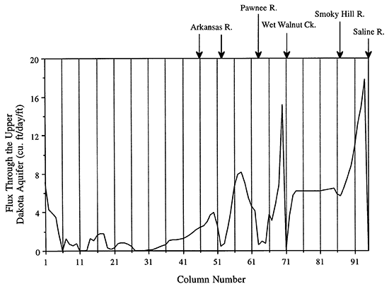
Flow rates within the upper part of the Dakota aquifer reflect the variability in recharge to and discharge from the model (compare Figures 6 and 7). Lateral flow rates the upper Dakota fluctuate and are low in southeastern Colorado and southwestern Kansas up to approximately column 36 in the model. This is because of recharge to and discharge from local flow systems and variability in aquifer thickness due to erosion. Beyond column 36 in the central Kansas part of the model, flow rates in the upper Dakota are higher but fluctuate dramatically as the flow rate and flow direction across the upper model boundary changes along the model.
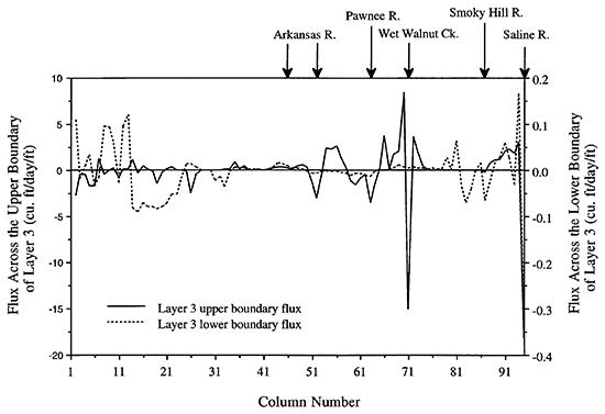
Figure 7--The lateral flux of water through the upper Dakota aquifer.
Though not as important, flow between the upper and lower Dakota aquifer across the Kiowa shale aquitard is also a factor (Figure 8). Small but significant flows occur from the upper to the lower Dakota in columns 1-13 of the model. In columns 12-17 the flow direction reverses and the lower Dakota provides recharge to the upper Dakota. Elsewhere in the model significant flows between these two aquifers occur from columns 80-95. Interestingly, upward flow from the lower Dakota is indicated beneath the Smoky Hill River in the area where the salinity begins to increase in the stream discharge. The lower Dakota is known to contain naturally-occurring saltwater in this part of Russell County, Kansas (Macfarlane et al., 1988).
Figure 8--Vertical fluxes across Layer 3 (upper Dakota aquifer) of the southern vertical profile model. Positive fluxes indicate downward flow and negative fluxes indicate upward flow.
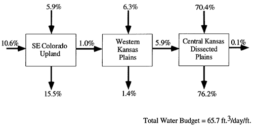
The water budget is summarized in Figure 9 and shows the distribution of recharge to and discharge from the upper part of the steady-state flow system for each of the three model sections listed in the earlier part of this report. The total water budget for the model is approximately 65.7 ft3/day through the 1 ft wide cross section. This is approximately four times the flow rate through the northern vertical profile model. The relative amounts of flow shown in the figure indicate that (1) very little flow moves between the various model sections, (2) most of the flow that enters the model is discharged locally, and (3) the majority of the water budget cycles through the model in the central Kansas section where the local flow systems dominate the regional system. Using the water budgets from both vertical profile models, it appears that most of the steady-state flow in the outcrop/subcrop region of the Dakota is of a local nature. It is an interesting outcome of the southern vertical profile model that only 6% of the total water budget or moves from the southwestern Kansas section of the model to the central Kansas section. In comparison, 70% of the total water budget enters this model section as recharge across the water table in central Kansas.
Figure 9--Overall water budget for the southern vertical profile model by model section. Percentages are of the total water budget for the model.
This interpretation of the upper part of the regional system is generally supported by the major ion ground-water geochemistry along the southern vertical profile. Bicarbonate type waters with low total dissolved solids concentrations (less than 500 mg/l) are the most common in the Dakota aquifer along the trace of the southern vertical profile. These chemical characteristics reflect recharge from infiltrated precipitation or the overlying High Plains aquifer (Robson and Banta, 1987).
The steady-state water budget of the upper part of the regional flow system in the northern vertical profile model is similar to budget for the southern vertical profile. In each instance, the active part of the flow system is in the regional recharge area and in the central Kansas model sections. In between, very little recharge is added to the model in the western and southwestern Kansas model sections, respectively because of low topographic relief. The major difference between the water budgets for each model is the much higher flow through the southern vertical profile model. Nearly four times as much water flows through the southern vertical profile as flows through the northern vertical profile. The increase in flow through the model and the upper Dakota (Figures 7 and 8) seems to be primarily because of (1) the improved hydraulic connection between the overlying water table and the Dakota aquifer and (2) the increase in Dakota aquifer transmissivity in the southern vertical profile model.
The primary goal of this part of the flow-system modeling was to compare the sensitivity of the northern and southern vertical profile models to vertical hydraulic conductivity or transmissivity of the major aquifer units. Sensitivity analysis can be used as a means to determine which parameters most influence flow-system dynamics. The effect of each hydrostratigraphic unit was evaluated by running series of simulations in which the hydraulic properties were varied systematically through a range of likely values. Values of the aquitard vertical hydraulic conductivity were selected over a range of plus or minus two or three orders of magnitude of the partially calibrated values for each cell by multiplying the parameter by the appropriate power of 10. For the aquifer units, the transmissivity was varied over a range of plus or minus 75% of the partially calibrated values for each cell by increments of 25%. The effect of changing the value of the parameter in each cell on the model was determined by calculating the RMS error after each model run using Eqn. 2. Plots of the percentage of the transmissivity or the multiplier of the vertical hydraulic conductivity in the partially calibrated model vs. the RMS error were prepared to show the effect of the layer parameter change on the head distribution (flow-system sensitivity).
Figure 10 shows the results of the sensitivity analysis for the vertical hydraulic conductivity of the Upper Cretaceous aquitard in both the northern and the southern vertical profile models. The change in RMS error is very small over the range of multipliers of vertical hydraulic conductivity tested in the southern vertical profile model. In comparison, the change in RMS error in the northern vertical profile model over the same range of multipliers is very large. This demonstrates that the flow system in the northern vertical profile is much more sensitive to the aquitard vertical hydraulic conductivity than the flow system in the southern vertical profile. The flow system in the southern vertical profile appears to be insensitive to this parameter because the aquitard is relatively thin and discontinuous in the profile (Figure 2). An additional factor is that the vertical hydraulic conductivity of this layer is on the average slightly higher in the southern vertical profile model than in the northern vertical profile model. In southwestern Kansas the aquitard has a vertical hydraulic conductivity of 9.0 x 10⁻⁵ ft/day and in the central Kansas section, 3.0 x 10⁻⁵ to 4.6 x 10⁻⁷ ft/day. The net effect of these differences is that the upper Dakota, which contains most of the target heads in the model, is not hydraulically isolated from the overlying water table over large areas of the model.
Figure 10--Model sensitivity to the Upper Cretaceous aquitard vertical hydraulic conductivity.
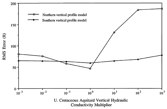
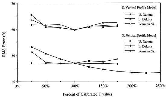
Figure 11 shows the results of the sensitivity analysis for aquifer transmissivity in both the northern and the southern vertical profile models. The results show that the hydraulic heads in both models are relatively insensitive to the aquifer transmissivity parameters.
Figure 11--Model sensitivity to aquifer transmissivity (T).
The regional potentiometric surface map of the Dakota aquifer in southeastern Colorado and Kansas suggests apparent regional recharge and discharge areas in southeastern Colorado and central Kansas. The vertical profile models show that there is a progressive change in the dominant influences on the regional flow system in western Kansas. The regional system is characterized by smaller scale systems which are superimposed on and progressively dominate the regional system as the outcrop/subcrop areas are approached. The progressive thinning of the Upper Cretaceous aquitard and the more pronounced local topographic relief in the outcrop/subcrop area changes the hydrology from a relatively sluggish, deep basinal regime in northwest Kansas to a more active, near-surface flow regime in central and southwestern portions of the state. In the northern vertical profile, the flow system in the upper Dakota is most influenced by the hydraulic isolation imposed by the Upper Cretaceous aquitard and the river valleys. Most of the recharge to the Dakota aquifer in western Kansas originates from southeastern Colorado. In contrast, the major influence on the flow system in the Dakota in the southern vertical profile model is topography. Most of the recharge to the Dakota aquifer is local in origin. The hydrostratigraphy has little influence on the key features of the flow system in this model.
Anderson, M.P., and Woessner, W.W., Applied groundwater modeling simulation of flow and transport: San Diego, Academic Press, 381 p.
Belitz, K., 1985, Hydrodynamics of the Denver basin: an explanation of subnormal fluid pressures: Ph.D. Thesis, Stanford University, Stanford, CA, 194 p.
Belitz, K., and Bredehoeft, J. D., 1988, Hydrodynamics of the Denver basin: explanation of fluid subnormal pressures: American Association of Petroleum Geologists Bulletin, 72(11), pp. 1334-1359.
Dugan, J.T., and Peckenpaugh, J.M., 1985, Effects of climate, vegetation, and soils on consumptive water use and ground-water recharge to the Central Midwest Regional Aquifer System, mid-continent United States: U.S. Geological Survey, Water-Resources Investigations Report 85-4236, 78 p. [available online]
Fenneman, N.M., 1946, Physical subdivisions of the United States (Map): U.S., Geological Survey, 1 :700,000, 1 sheet.
Freeze, R.A., and Witherspoon, P.A., 1967, Theoretical analysis of regional ground-water flow: 2. effect of water-table configuration and subsurface permeability variation: Water Resources Research, 3, pp. 623-634.
Harbaugh, A.W., 1990, A computer program for calculating subregional water budgets using results from the U.S. Geological Survey modular three-dimensional finite-difference ground-water flow model: U.S. Geological Survey, Open-file Report 90-392, 46 p. [available online]
Helgesen, J.O., Leonard, R.B., and Wolf, R.J., 1993, Aquifer systems underlying Kansas, Nebraska, and parts of Arkansas, Colorado, Missouri, New Mexico, Oklahoma, South Dakota, Texas, and Wyoming--hydrology of the Great Plains aquifer system in Nebraska, Colorado, Kansas, and adjacent areas: U.S. Geological Survey, Professional Paper 1414-E, 161 p. [available online]
Helgesen, J.O., Jorgensen, D.G., Leonard, R.B., and Signor, D.C., 1982, Regional study of the Dakota aquifer (Darton's Dakota revisited): Ground Water, 20(4), pp. 410-414.
Hershey, L.A., and Hampton, E.R., 1974, Geohydrology of Baca and southern Prowers counties, southeastern Colorado: U.S. Geological Survey, Water Resources Investigations 16-74, 1 sheet. [available online]
Jordan, P.R., Jones, B.F., and Petri, L.R., 1964, Chemical quality of surface waters and sedimentation in the Saline River basin Kansas: U.S. Geological Survey, Water Supply Paper 1651, 90 p. [available online]
Leonard, R.B., Signor, D.C., Jorgensen, D.G., and Helgesen, J.O., 1983, Geohydrology and hydrochemistry of the Dakota aquifer, central United States: Water Resources Bulletin, 19(6), pp. 903-911.
Macfarlane, P.A., Townsend, M.A, Whitemore, D.O., Doveton, J.H., and Staton, M., 1988, Hydrogeology and water chemistry of the Great Plains (Dakota, Kiowa, and Cheyenne) and Cedar Hills aquifers in central Kansas--end of contract report: Kansas Geological Survey, Open-file Report 88-39, 184 p. [available online]
Macfarlane, P.A., Whittemore, D.O., Townsend, M.A., Doveton, J.H., Hamilton, V.J., Coyle III, W.G., Wade, A., Macpherson, G.L., and Black, R.D., 1990, The Dakota Aquifer Program: annual report, FY89: Kansas Geological Survey, Open-file Report 90-27, 301 p. [available online]
Macfarlane, P.A., and , Chu, T., Butler, J.J., Jr., Wade, A., Coleman, J., Doveton, J.H., Mitchell, J., and Kay, S., 1992, The Dakota Aquifer Program: annual report, FY91: Kansas Geological Survey, Open-file Report 92-1, 93 p. [available online]
Macfarlane, P.A., 1993, The effect of topographic relief and hydrostratigraphy on the upper part of the regional ground-water flow system in southeastern Colorado and western and central Kansas, with emphasis on the Dakota aquifer: Ph.D Dissertation, University of Kansas, Lawrence, KS, 197 p.
McDonald, M.G., and Harbaugh, A.W., 1988, A modular three-dimensional finite-difference ground-water flow model: U.S. Geological Survey, Techniques of Water Resources Investigations, Book 6, Chapter A1, 576 p.
McLaughlin, T.G., 1954, Geology and groundwater resources of Baca County, Colorado: U.S. Geological Survey, Water Supply Paper 1256, 232 p. [available online]
Robson, S.G., and Banta, E.R, 1987, Geology and hydrology of deep bedrock aquifers in eastern Colorado: U.S. Geological Survey, Water-Resources Investigations Report 85-4240, 6 sheets. [available online]
Stullken, L.E., and Pabst, M.E., 1982, Altitude and configuration of the water table in the High Plains aquifer of Kansas, pre-1950 (map): U.S. Geological Survey, Open-file Report 82-117, 1 sheet. [available online]
Toth, J., 1962, A theory of groundwater motion in small drainage basins in central Alberta, Canada: Journal of Geophysical Research, 67(11) pp. 4375-4387.
Toth, J., 1963, A theoretical analysis of groundwater flow in small drainage basins: Journal of Geophysical Research, 68, pp. 4795-4812.
Kansas Geological Survey, Geohydrology
Placed online Feb. 24, 2016; originally released 1996
Comments to webadmin@kgs.ku.edu
The URL for this page is http://www.kgs.ku.edu/Hydro/Publications/1996/OFR96_1d/index.html