Kansas Geological Survey, Open-file Rept. 95-1a
Next--Appendices
Originally released in 1995 as Kansas Geological Survey Open-file Rept. 95-1a. Special problem report CE 890. This is, in general, the original text as published. The information has not been updated. An Acrobat PDF version (25 MB) is also available.
A contoured map of total dissolved solids was prepared using water resistivity values calculated from the self potential curve of geophysical logs for sands in the Dakota aquifer in northwest Kansas. Water resistivities were calculated using the self potential curve from wells that had actual water resistivity measurements or were near wells that had actual measurements. The calculated resistivities were plotted versus actual measured resistivities to develop an empirically derived Dakota Aquifer type curve. A polynomial equation was determined for the line of best fit for the empirically derived curve. Geophysical logs from 977 boreholes in 11 counties were used to estimate water resistivity for sand units in the Dakota aquifer of northwest Kansas. The polynomial equation was used to correct these values to yield better estimates of actual water resistivity. The corrected resistivity values were converted to specific conductivity and then to total dissolved solids using a previously established empirical relationship between specific conductivity and total dissolved solids for the Dakota Aquifer.
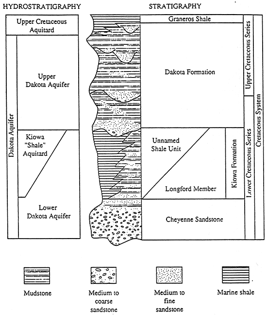
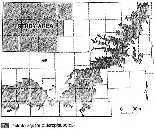
The Dakota Aquifer as outcrop and in the subsurface covers roughly the western half of Kansas (Figure 1). The Dakota aquifer is composed of interbedded sandstones and shales that were deposited in river valleys, deltas, and nearshore marine environments (McFarlane et al., 1991). It is the second most geographically extensive aquifer system in Kansas after the High Plains aquifer (Ogallala and associated alluvial aquifers) (Mcfarlane et al., 1990). Presently the Dakota aquifer is used widely for irrigation, public water supplies and industry in southwest, south central and north central Kansas where the aquifer is relatively shallow (McFarlane et al., 1990). The Dakota aquifer in Kansas consists of the Dakota Formation, Kiowa Formation, and the Cheyenne Sandstone (Figure 2) (McFarlane et al., 1990). This project is primarily concerned with the Dakota Formation as it generally contains sands with better water quality than the Kiowa Formation and Cheyenne Sandstone.
Figure 1--Extent of the Dakota aquifer in Kansas.
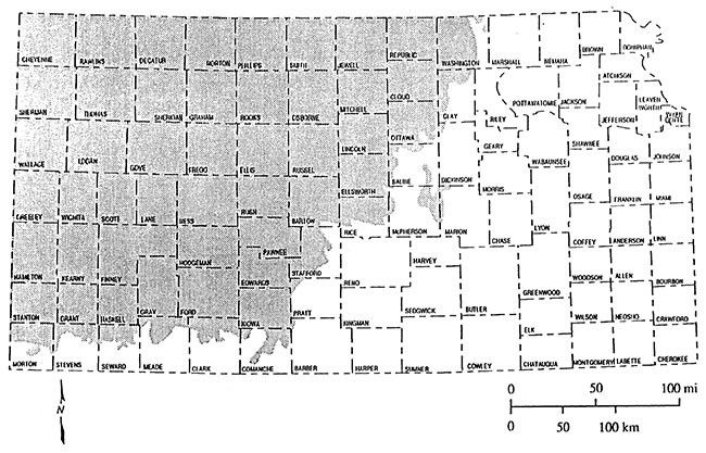
Figure 2--Stratigraphic and hydrostratigraphic classification of units that compose the Dakota aquifer in Kansas.
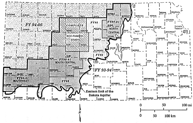
This project was coordinated with the Kansas Geological Survey Dakota aquifer program. The Dakota aquifer program is an eight year study which began in 1989 (figure 3). The program goals are to provide a better understanding of the Dakota aquifer's geologic framework, hydrogeology, and hydrogeochemistry. This information can be used to help state water planning and regulatory agencies evaluate the aquifer as a future source of water for central and western Kansas (McFarlane et al., 1989).
Figure 3--Subareas of investigation in the Dakota aquifer program.
This study is part of years 6,7, and 8 of the project and covers all or portions of eleven counties located in the northwest corner of the state (figure 4).
Figure 4--Study Area
In the near future, localized depletion of the High Plains aquifer in western areas of Kansas and depletion of water supplies in the stream aquifer system in the central part of the state may cause critical water shortages (McFarlane et al., 1990). The cities of Hays and Russell in west central Kansas have already drilled wells to evaluate the quality and quantity of Dakota waters. The city of Hays is currently using its Dakota well field for municipal and domestic water supplies.
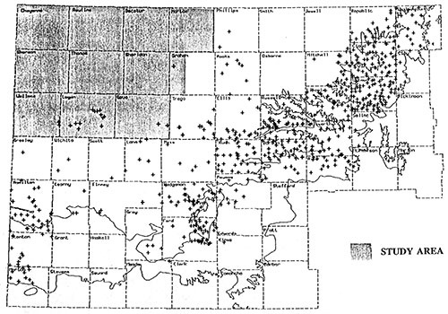
Except for scattered wells located along the eastern and southern portions of the study area there is no existing water quality information for the Dakota aquifer in northwest Kansas (figure 5). This study will provide a better estimate of water quality in the Dakota aquifer in the northwestern part of the State.
There were four main objectives of the study: 1) to estimate water quality in the Dakota aquifer of northwest Kansas by estimating total dissolved solids; 2) to combine this data with existing maps to produce updated and more accurate water quality maps; 3) to determine where the Dakota aquifer contains fresh water (<1,000 mg/l TDS) and areas where the Dakota waters must be protected per requirements of the Kansas Corporation Commission (<10,000 mg/l TDS); and 4) to provide data to the Dakota aquifer program which can be combined with geological studies and other studies to determine the best potential areas for further investigation with regard to water quality and quantity.
Figure 5--Existing Dakota Water Quality Database
The methodology used to determine the estimated total dissolved solids of Dakota aquifer waters was as follows:
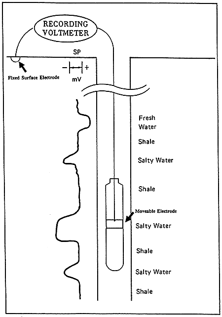
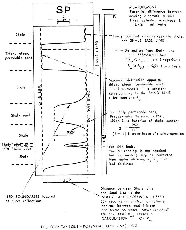
The SP curve is a recording versus depth of the potential difference between a moveable electrode in the borehole and a fixed surface electrode measured in millivolts (Figure 6). This battery is created by salinity (resistivity) contrasts between formation waters and the mud used in drilling operations. The Drilling process juxtaposes two solutions, the mud filtrate and formation water, with different ion concentrations. The difference in ion concentrations causes ions to diffuse from the more concentrated solution to the more dilute solution. This ion flow has an associated potential measured in millivolts.
Figure 6--General illustration of SP Log (After Dresser Atlas Publications)
The deflection of the SP recording corresponds to the potential differences created in the mud by the SP currents and make it possible to characterize formations (Franks, 1986). The main uses of the SP are to delineate porous and permeable beds and to determine formation water resistivity.
The cumulative potential is generated by electromotive forces (emf) generally of electrochemical and electrokinetic origins. The electrochemical components are the membrane potential and the liquid-junction potential.
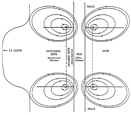
Figure 7 shows a permeable sand invaded by mud filtrate and sandwiched between two thick shale beds. The membrane potential occurs at the contact between the drilling fluids in the pores of a permeable bed and the adjacent shales. Because of the layered clay structure and the charges on the layers, shales are ion selective and permeable to the Na+ cations but impervious to the Cl- anions. Only the Na+ cations are able to move through the shale from the more concentrated to the less concentrated NaCl solution (Schlumberger, 1987).
Figure 7--Membrane and Liquid Junction Potentials (After Schlumberger Publications)
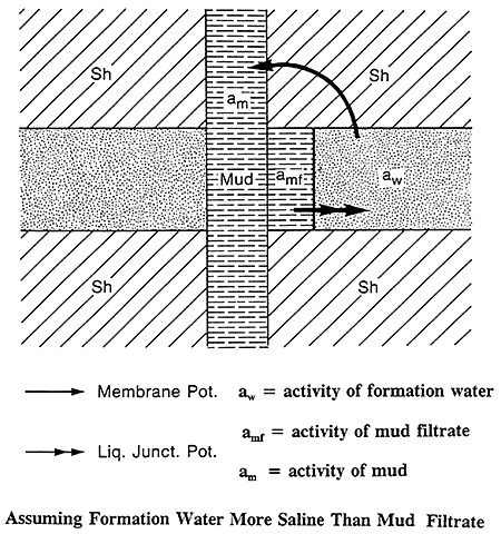
The liquid-junction potential occurs at the edge of the invaded zone, where the mud filtrate and formation water are in direct contact. Na+ and Cl- are free to diffuse from the more concentrated solution to the less concentrated. Chloride ions are more mobile and the net result of this ion diffusion is flow of Cl- ions from the more concentrated solution to the less concentrated solution. This is equivalent to a conventional current flow in the opposite direction (Schlumberger, 1987). The arrows in Figure 7 show the direction of the current flow assuming the formation water is more saline than the mud filtrate.
Figure 8 is a general illustration of currents associated with the membrane and liquid junction potentials. The resultant deflection of the SP curve is also shown. This drawing assumes the formation water is more saline than the mud filtrate.
Figure 8--SP Current Distribution (After Dresser Alias Publications)
The electrokinetic potential is usually small, and regarded as negligible (Schlumberger, 1987).
Calculating formation water resistivity from SP readings works better in sand/shale sequences with thick clean sands as they typically have higher porosities and permeabilities, lower resistivities and limited invasion profiles.
Usually the SP recording includes a shale baseline which is more or less straight and has deflections to the left or right adjacent to permeable beds. The SP tends to reach an essentially constant deflection opposite clean, porous, and permeable beds and this is known as the sand line (Figure 9). Also shown in Figure 9 are three resistivity curves to the right of the SP curve. Different resistivity measurements are usually presented along with the SP recording. These measurements are a function of the formation water and/or drilling fluid and the porosity of the adjacent rock. The difference between the shale line and the sand line is the maximum potential which can exist and is known as the static SP or the SSP. The SSP is the total sum of all the electrochemical forces.
Figure 9--Example of Sand and Shale Lines in a Sand-Shale Sequence (After Schlumberger Publications)
In sand/shale sequences with thick clean porous sands the magnitude and direction of the SP Curve is a function of the salinity contrast between the mud filtrate and formation water. Since salinity and resistivity are inversely related the SP is also a function of the resistivity contrast between the mud filtrate (Rmf) and the formation water (Rw) (Figure 10). The direction of the deflection follows these relationships:
Rmf > Rw: negative deflection, formation water more saline.
Rmf < Rw: positive deflection, filtrate water more saline.
Rmf = Rw: no deflection, equal salinities.
Figure 10--Examples of SP Deflection (After Asquith)
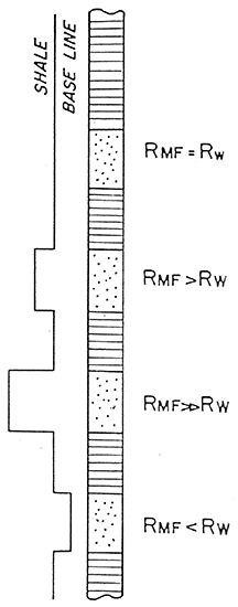
Figure 11 is a summary of the SP log.
Figure 11--Summary of SP Curve (After Doveton)
Based on laboratory tests and theoretical considerations published in numerous documents the total electrochemical emf, Ec, corresponding to the membrane potential plus the liquid junction potential, is represented by:
Ec = - K log (aw / amf)
with aw and amf being the activities at formation temperature of the formation water and mud filtrate respectively. K is a coefficient proportional to the absolute temperature. For NaCl solutions, K = 60 + (.133 x formation temp in °F) (Schlumberger, 1987). For NaCl solutions that are not extremely concentrated and do not contain other salts in appreciable amounts, formation water resistivities are inversely proportional to activities (Schlumberger, 1987); and since Ec = SSP the equation becomes:
SSP = - K log (Rmf / Rw)
For very salty formation waters where Rw < .1 ohm-m at 75° (>60,000 mg/l TDS for the Dakota) and for fresher waters where Rw > .3 ohm-m at 75° (<20,000 mg/l TDS for the Dakota) the inverse proportion does not hold exactly and values of K may differ from calculated values (Schlumberger, 1987). Highly saline waters are typically encountered when drilling for oil and gas and widely accepted corrections to Rw calculations have been extensively published. Corrections for fresh waters have not been the focus of as much research and there are no accepted correction formulas.
Fresher waters have significant amounts of Ca+2 and Mg+2 cations and the SSP value is then represented mathematically as:
SSP = - K log [(aNa +(aCa + aMg)1/2)w /(aNa +(aCa + aMg)1/2)mf]
where aNa, aCa, and aMg are the ionic activities of Na, Ca, and Mg in the formation water and the mud filtrate (Schlumberger, 1987). The effect of Ca+2 and Mg+2 on the SP is to lower the deflection (Schlumberger, 1987). This effect makes the calculation of the formation water resistivity lower than the actual resistivity (water will appear to be more saline than it actually is). Since the inverse relationship between activities and resistivities is not exact in this instance equivalent resistivities Rwe and Rmfe are used and the equation becomes:
SSP = - K log (Rmfe/Rwe)
Equivalent resistivities are calculated resistivities assuming the water is a NaCl solution. This is the important deviation point that must be accounted for in evaluating fresh water zones.
From the above equation it can be seen that if the SSP, K, and Rmfe values are known, Rwe can be determined. The values needed can be obtained or calculated from information on the log heading and in the case of the SSP, directly from the log presentation. Rmfe values are determined using established empirical relationships (Schlumberger, 1987). The following steps are used to determine Rwe:
Retrieve from log:
Procedure:
The standard temperature of 75°F is used in the oil and gas industry for which log interpretation methods are primarily focused. The correction to 77°F is made to correspond with the standard temperature used in the water industry.
Volumes have been written on obtaining Rw from Rwe in saline waters as these are typically encountered while drilling for oil and gas. In fresh water zones it is critical to establish empirical relationships between Rwe and actual Rw values in order to make better estimations of water quality. The main objective of this paper is to determine this empirical relationship for the Dakota aquifer using a limited number of observations and to use this relationship to correct Rwe values to obtain better estimates of actual water resistivities.
In 1956 Gondouin et al. studied the influence of other salts on SP logs to explain why abnormal readings were observed in fresh water and highly saline zones. They investigated the influence of HCO3-, SO4-2, Ca+2, and Mg+2 on the magnitude of the SP deflection. It was determined that the effect of HCO3- and SO4-2 on the activity of Na+ was negligible when Na+ was the predominant cation. Ca+2 and Mg+2 cations were found to have a relatively large influence on the SP.
An empirical relationship between Rwe calculated from SP logs and actual formation water resistivities (Rw) was established for a combination of fresh waters in Venezuela, Nebraska, Colorado, and California. Field studies confirmed that empirically corrected Rw values calculated from the SP were generally within 10% of actual Rw readings from produced waters. Gondouin et al. recommended that for low salinity waters local plots of Rwe versus Rw be used to gain greater accuracy in determining water quality from the SP.
Alger in 1966 used empirical methods to show that good results could be obtained in estimating total dissolved solids and chloride concentrations in fresh water using the SP. Alger developed an empirical relationship for Rwe values calculated from the SP and actual fresh water resistivities for four Texas gulf coast aquifers. Alger also stated that relative ion assemblages are reasonably predictable on a local basis and this allows empirical studies to determine estimated total dissolved solids and chloride concentrations from computed values of Rw.
McConnell in 1983 used the SP to compute the thickness and distribution of groundwater with total dissolved solids of less than 1000 mg/l (ppm) in the Garber Sandstone and Oscar Group in Carter County, Oklahoma. McConnel states that when Ca+2 and Mg+2 are present an empirical relationship between Rwe and Rw must be developed for that particular local water chemistry and used as a correction factor.
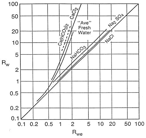
Schlumberger (1987) states that in fresh water formations salts other than NaCl may become important. In these cases, the Rwe-Rw relationship may be quite different from that for NaCl dominated waters and empirical Rwe-Rw charts should be developed. Figure 12 is a Schlumberger graph showing theoretical Rwe-Rw curves at 77°F for solutions of several different salts and the area where plots for average fresh waters would be.
Figure 12--Rw vs. Rwe for Solutions of Different Salts
A paper with no stated author or year of publication was supplied to the author by P.A. McFarlane. From references cited it is estimated the date of publication was in the early 1960's. The publication estimated the salinity of groundwater in the Cheyenne Formation of Northwestern Kansas. The author used both the resistivity ratio method and the SP method to calculate formation water resistivity. The only use the author made of the SP derived resistivities was to compare them with resistivities derived from long and short normal resistivity curves.
The author created an empirical correction curve for the Cheyenne by plotting measured resistivities of Dakota waters from 15 wells in Nebraska and Colorado versus resistivities calculated from long and short normal curves using the ratio method. (For explanation of the ratio method using long and short normal curves see Franks, 1986). The Dakota was used instead of actual Cheyenne water as no analyses of Cheyenne waters were available. Maps showing estimated salinities in the Cheyenne formation in western Kansas were generated using only the resistivity derived resistivities converted to salinities using charts published by Schlumberger.
The significance of this paper is that it was an early attempt to determine water quality from logs in western Kansas using Dakota aquifer water analyses.
The best and most recent estimates of water quality in the Dakota aquifer in northwest Kansas are presented in maps prepared by Dr. Don Whittemore of the Kansas Geological Survey. Figure 13 is a total dissolved solids map prepared by Dr. Whittemore prior to this study. Water quality in most of the study area was estimated using maps prepared by the United States Geological Survey and limited available water analyses.
Figure 13--Kansas Geological Survey Dakota Aquifer Total Dissolved Solids Map.
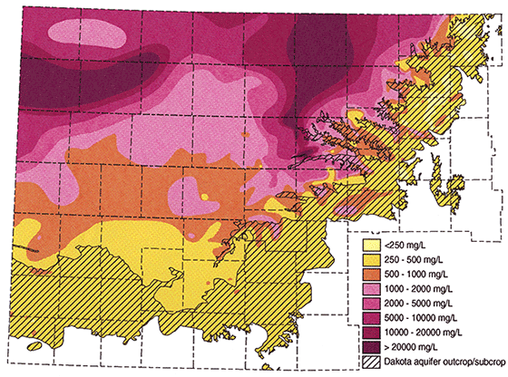
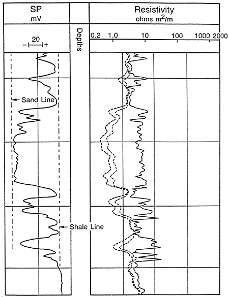
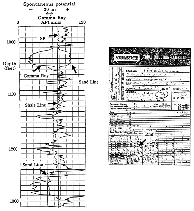
Figure 14 is an example of a geophysical log across a portion of the Dakota aquifer. There are two thick clean sands on this log. The upper sand from 1015-1045 exhibits a positive SP deflection. The lower sand from 1255-1288 exhibits a negative SP deflection. Sample calculations will be made for both sands. Four data entries are obtained from the log itself. Rmf, Rmf temperature, formation depth and the SSP. The Rmf and Rmf temperature can be retrieved directly from the log heading. In this example, Rmf = 1.08 at 75°F. Notice that there are two Rmf values on this log. The one made at 75°F is probably the actual measured value and the one at 105°F has probably been calculated from the measured value. It is not common to have the Rmf value given at 75°F on the log heading and a conversion is usually necessary. Formation depths are retrieved from the log track. To obtain the SSP the shale and sand lines are drawn. The magnitude is measured using the scale at the top of the SP log track. In this example each chart division = 20 millivolts. The associated equations and computer program used to convert this data into Rwe are presented in Appendix A.
| Upper Sand | Lower Sand | |
|---|---|---|
| Rmf (from log heading) | 1.08 at 75°F | 1.08 at 75°F |
| Formation Depth | 1030' | 1265' |
| SSP | 40 mv | -36 mv |
| Formation Temperature (Ave. Temp Gradient Method) | 70°F | 74°F |
| Rmf at 75° F (Arp's equation if necessary) | 108 | 108 |
| K at formation temperature | 69.31 | 68.842 |
| Rmfe at 75°(empirical studies) | .918 | .918 |
| Rmfe/Rwe | .2751 | 3.3577 |
| Rwe at 77° | 3.3803 | .2734 |
Figure 14--Sample Calculation Log
Rwe = Rw for waters that are not extremely saline or fresh. Rwe values for fresh waters have to be corrected by an empirically derived equation determined by plotting Rwe values versus actual resistivity values.
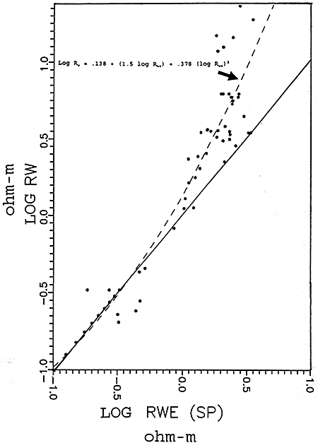
To determine the empirical relationship between Rwe and Rw, water quality data for 28 wells in 16 different areas were supplied by Dr. Don Whittemore of the Kansas Geological Survey (Figure 16). Fourteen wells had analyses for two sands for a total of 42 measured water quality data points. Thirty nine of the data points are from the Dakota, two from the Cheyenne and one from the Cedar Hills. Sixteen of the twenty eight wells had a geophysical log with a SP from the same borehole. For the remaining twelve wells the closest possible well(s) with an SP log was retrieved for calculating Rwe. Where the stratigraphy was not identical between the measured well and the nearby well a sand close to the same interval within the Dakota was selected. Of these 12 wells seven had the measured value plotted versus one nearby calculated Rwe. One well's measured resistivity was plotted versus four nearby Rwe values. Two well's resistivities were plotted versus two nearby Rwe values each. Two measured values from different sands from the same well were plotted versus five nearby Rwe values from two nearby wells. One well was plotted versus an average of four different sands from a nearby well. In all, fifty measured water quality data points were used to determine the empirical relationship. Appendix B shows the data in tabular form.
Figure 16 is the graphical representation of the empirical data. This graph was generated using log values rather than the actual resistivity values. This graph shows the line of best fit and the calculated polynomial equation for the line. Most of the data used to determine the empirical relationship were in the fresh water range. Nine extra data points were plotted in the salt water region of the chart (.1 - .3 ohm-m)(-.1 to -.5 ohm-m log values). This was done for two purposes: 1) to make the graph go through the intersection of the graph axes, as a linear relationship should exist in the higher salinity region of the graph; and 2) to include the influence of salt water zones in the calculation of the empirical relationship. The difference between using the additional nine points and not using them is shown in Table 1.
Figure 15--Map Showing Empirical Database Locations
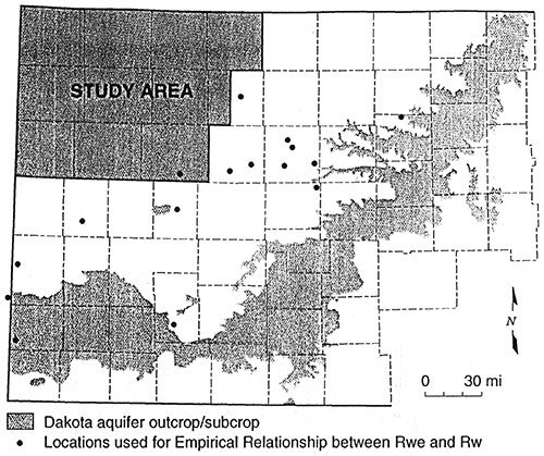
Figure 16--Empirical Rw vs. Rwe Graph
The empirical relationship between specific conductivity (resistivity) and total dissolved solids was supplied by Dr. Whittemore of the Kansas Geological Survey. This relationship was determined from a large database from actual Dakota aquifer waters. At 77°F:
TDS = .6 x Specific Conductivity (SC = 10000 / Rw)
Applying the empirically derived equation to the log presented in the sample calculation on page 28 the results would be:
| Upper Sand | Lower Sand | |
|---|---|---|
| Rmfe/Rwe | .2751 | 3.3577 |
| Rwe at 77° | 3.3803 | .2734 |
| Rwat 77° | 10.0000 | .2546 |
The comparison between TDS for Rwe and Rw is:
| Upper Sand TDS mg/l |
Lower Sand TDS mg/l |
|
|---|---|---|
| Rwe | 1774 | 21,945 |
| Rw | 550 | 23,172 |
Table 1--Comparison of Equations
|
Empirical Equation Using Extra Nine Data Points Log Rw = .138 + 1.5 log Rwe + .378 (log Rwe)2 Empirical Equation Not Using Extra Nine Data Points Log Rw = .142 + 1.51 log Rwe + .311 (log Rwe)2 |
| Comparison of TDS Results at Different Salinities | |||
| Assumed Rwe | Extra Nine Equation |
Original Equation |
|
|---|---|---|---|
| 1) | 5 ohm-m | 255 mg/l | 268 mg/l |
| 2) | 3 ohm-m | 689 mg/l | 700 mg/l |
| 3) | 1 ohm-m | 4,366 mg/l | 4,325 mg/l |
| 4) | .5 ohm-m | 11,413 mg/l | 11,549 mg/l |
| 5) | .3 ohm-m | 20,949 mg/l | 21,905 mg/l |
| 6) | .2 ohm-m | 31,880 mg/l | 34,602 mg/l |
| 7) | .15 ohm-m | 41,637 mg/l | 46,656 mg/l |
Appendix C contains the tabular presentation of the retrieved and calculated data for all logs used to create the Dakota water quality database. Figure 17 is a map showing the location of these data points. A total of 977 logs were used to create the database. Rw values were calculated for one sand for 890 boreholes, two sand units at different depths for 69 boreholes, three sand units for 14 boreholes, and four sand units for 4 boreholes, for a total of 1086 calculated values. 1078 values are for Dakota Formation sands, 3 for sands in the Kiowa Formation and 5 for sands in the Cheyenne Sandstone. Only one data entry was made for each well to produce the final maps.
When more than one thick clean porous sand was seen on a log the sand which contained the freshest water by calculation was used for producing the maps. Values for other sands were calculated for comparison purposes only.
Figure 17--SP Derived Water Quality Database
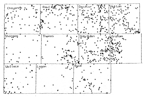
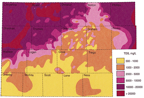
Figure 18 is the final contoured map of the estimated total dissolved solids in Dakota Formation waters in northwest Kansas. The map was combined with Dr. Whittemore's map to produce the final map and includes the neighboring counties on the southern and eastern edges of the study area.
Figure 18--Dakota aquifer Total Dissolved Solids map
The empirical relationship between Rwe and Rw calculated for the Dakota aquifer using Spontaneous Potential logs was patterned after methods previously published by Gondouin, Alger, and Schlumberger Logging Services. These studies determined that empirical relationships should be used to better estimate formation water resistivities in low salinity waters. The empirical relationship established for the Dakota aquifer confirmed that the fresher waters become the greater the difference between SP calculated formation water resistivities and measured resistivities.
The graphical presentation of the Dakota aquifer empirical data (Figure 17) fits into the area of "average" fresh waters as presented in the Schlumberger graph on page 24. Comparing the Schlumberger graph with the Dakota aquifer empirical graph, three observations can be made.
On the Dakota aquifer graph it is observed that for formation waters in the .4 to .7 log Rw range a number of data points fall beneath the line of best fit. These data points may represent data calculated from predominately NaHCO3 or Na2SO4 waters. The Schlumberger graph shows that the theoretical NaHCO3 and Na2SO4 lines lie just above the NaCl single salt solution line. This indicates that Rwe values for waters where the predominate salt is NaHCO3 or Na2SO4 would plot closer to the single salt NaCI line and away from the line of best fit for all Dakota waters. The result of this observation is that for predominately NaHCO3 and Na2SO4 waters the empirical equation would calculate optimistic values for TDS concentrations.
In the freshest area of the graph (1.0+ log Rw values) the data points fall above the line of best fit. This is probably the result of these waters being predominately CaCl2, MgCl2, Ca(HCO3)2, or Mg(HCO3)2 waters and would tend to plot towards the CaCl2 line on the Schlumberger graph. The result of this observation is that for very fresh waters the empirical equation would yield pessimistic values.
In the highly saline portion of the graph (<-.5 log Rw) the few empirical data points available do not fit the theoretical single salt solution line. Of the eight data points used in the more saline portion of the graph three data points lie very close to the line while five are scattered. Of the five, the four that fall below the line are from the same well and some other factor associated with the mud or logging tools could be playing a part in this deviation. Without using the nine artificial data points the four data points below the line would have a large influence on the calculations of TDS for highly saline waters. This effect is illustrated in Table 1 on page 34. This scatter is not significant as waters in this range typically have TDS values >15,000 to 20,000 mg/l, and a 10-15% correction factor is not important as the water is of such poor quality.
The final result of this study was the TDS concentration map. Besides being colorful and interesting to look at, just what does this map mean? The map shows the typical TDS concentrations that would probably be encountered in the Dakota Formation in the northwest portion of Kansas. If an individual or municipality wanted to drill for water in the Dakota Formation, the map could be use to estimate the water quality that might be encountered at the location of interest. The map provides an estimate of the freshest water that might be found in the Dakota Formation and should be used as a general reconnaissance tool.
The two critical areas of the TDS map are the area of fresh water (<1000 mg/l TDS) and the area where the Dakota aquifer must be protected (<10,000 mg/l). The <1000 mg/l area is predominately restricted to the southern portions of the study area in Logan, and Gove counties. There is a large area in Sheridan, Graham, and Gove counties where the general TDS range is between 1000-2000 mg/l. Within this area there are areas where the Dakota may contain waters with TDS in the 500-1000 mg/l as well as areas where TDS might be in the 2000-5000 mg/l range. The reason for this variance probably lies in the geology of the Dakota Formation. Throughout this area a thick porous basal channel sand is often encountered. Where this sand is present it usually calculates to have fresher water than the shallower thinner and less porous Dakota sands. The areas where fresher waters are projected are most likely areas where the basal channel sand was present and used in the calculations. The areas where the projected TDS values are higher are most likely areas where the basal channel sand was absent and shallower sands were used in the calculations. When looking for potential areas to drill for Dakota waters in this area it would be important to combine this map along with a complete geological study. It is projected that a complete geological study would result in a map which would project where these paleochannels are most likely present.
The <10,000 mg/l line runs SW - NE through Wallace, Logan, Thomas, Sheridan, Decatur, and Norton counties. To the south and southeast of this line the potential exits for encountering Dakota waters which must be protected. There are some areas to the north of this line which may have waters that need to be protected but the calculations are near the 10,000 mg/l level and more data are needed to definitely say that the Dakota needs protection in these areas.
On the original map provided by Dr. Whittemore there was a large area in Cheyenne county that was shown to have <10,000 mg/l TDS. This study does not confirm this speculation and it is not recommended that the Dakota waters be protected this far west.
It is believed that the amount and quality of the data collected should greatly help with the prediction of water quality in the Dakota Formation in western Kansas. It is hoped that these data can be combined with other water quality and geological studies to help in better understanding the potential role the Dakota aquifer might play in augmenting the useable water resources of Kansas.
Kansas Geological Survey, Geohydrology Section
Placed on web Aug. 19, 2014; originally published in 1999.
Comments to webadmin@kgs.ku.edu
The URL for this page is http://www.kgs.ku.edu/Publications/Bulletins/TS13/index.html